Popular searches
- How to Get Participants For Your Study
- How to Do Segmentation?
- Conjoint Preference Share Simulator
- MaxDiff Analysis
- Likert Scales
- Reliability & Validity

Request consultation
Do you need support in running a pricing or product study? We can help you with agile consumer research and conjoint analysis.
Looking for an online survey platform?
Conjointly offers a great survey tool with multiple question types, randomisation blocks, and multilingual support. The Basic tier is always free.
Research Methods Knowledge Base
- Navigating the Knowledge Base
- Foundations
- Measurement
- Research Design
- Conclusion Validity
- Data Preparation
- Descriptive Statistics
- Dummy Variables
- General Linear Model
- Posttest-Only Analysis
- Factorial Design Analysis
- Randomized Block Analysis
- Analysis of Covariance
- Nonequivalent Groups Analysis
- Regression-Discontinuity Analysis
- Regression Point Displacement
- Table of Contents
Fully-functional online survey tool with various question types, logic, randomisation, and reporting for unlimited number of surveys.
Completely free for academics and students .
The t-test assesses whether the means of two groups are statistically different from each other. This analysis is appropriate whenever you want to compare the means of two groups, and especially appropriate as the analysis for the posttest-only two-group randomized experimental design .
Figure 1 shows the distributions for the treated (blue) and control (green) groups in a study. Actually, the figure shows the idealized distribution – the actual distribution would usually be depicted with a histogram or bar graph . The figure indicates where the control and treatment group means are located. The question the t-test addresses is whether the means are statistically different.
What does it mean to say that the averages for two groups are statistically different? Consider the three situations shown in Figure 2. The first thing to notice about the three situations is that the difference between the means is the same in all three . But, you should also notice that the three situations don’t look the same – they tell very different stories. The top example shows a case with moderate variability of scores within each group. The second situation shows the high variability case. the third shows the case with low variability. Clearly, we would conclude that the two groups appear most different or distinct in the bottom or low-variability case. Why? Because there is relatively little overlap between the two bell-shaped curves. In the high variability case, the group difference appears least striking because the two bell-shaped distributions overlap so much.
This leads us to a very important conclusion: when we are looking at the differences between scores for two groups, we have to judge the difference between their means relative to the spread or variability of their scores. The t-test does just this.
Statistical Analysis of the t-test
The formula for the t-test is a ratio. The top part of the ratio is just the difference between the two means or averages. The bottom part is a measure of the variability or dispersion of the scores. This formula is essentially another example of the signal-to-noise metaphor in research: the difference between the means is the signal that, in this case, we think our program or treatment introduced into the data; the bottom part of the formula is a measure of variability that is essentially noise that may make it harder to see the group difference. Figure 3 shows the formula for the t-test and how the numerator and denominator are related to the distributions.
The top part of the formula is easy to compute – just find the difference between the means. The bottom part is called the standard error of the difference . To compute it, we take the variance for each group and divide it by the number of people in that group. We add these two values and then take their square root. The specific formula for the standard error of the difference between the means is:
Remember, that the variance is simply the square of the standard deviation .
The final formula for the t-test is:
The t -value will be positive if the first mean is larger than the second and negative if it is smaller. Once you compute the t -value you have to look it up in a table of significance to test whether the ratio is large enough to say that the difference between the groups is not likely to have been a chance finding. To test the significance, you need to set a risk level (called the alpha level ). In most social research, the “rule of thumb” is to set the alpha level at .05 . This means that five times out of a hundred you would find a statistically significant difference between the means even if there was none (i.e. by “chance”). You also need to determine the degrees of freedom (df) for the test. In the t-test , the degrees of freedom is the sum of the persons in both groups minus 2 . Given the alpha level, the df, and the t -value, you can look the t -value up in a standard table of significance (available as an appendix in the back of most statistics texts) to determine whether the t -value is large enough to be significant. If it is, you can conclude that the difference between the means for the two groups is different (even given the variability). Fortunately, statistical computer programs routinely print the significance test results and save you the trouble of looking them up in a table.
The t-test, one-way Analysis of Variance (ANOVA) and a form of regression analysis are mathematically equivalent (see the statistical analysis of the posttest-only randomized experimental design ) and would yield identical results.
Cookie Consent
Conjointly uses essential cookies to make our site work. We also use additional cookies in order to understand the usage of the site, gather audience analytics, and for remarketing purposes.
For more information on Conjointly's use of cookies, please read our Cookie Policy .
Which one are you?
I am new to conjointly, i am already using conjointly.
An open portfolio of interoperable, industry leading products
The Dotmatics digital science platform provides the first true end-to-end solution for scientific R&D, combining an enterprise data platform with the most widely used applications for data analysis, biologics, flow cytometry, chemicals innovation, and more.

Statistical analysis and graphing software for scientists
Bioinformatics, cloning, and antibody discovery software
Plan, visualize, & document core molecular biology procedures
Electronic Lab Notebook to organize, search and share data
Proteomics software for analysis of mass spec data
Modern cytometry analysis platform
Analysis, statistics, graphing and reporting of flow cytometry data
Software to optimize designs of clinical trials
The Ultimate Guide to T Tests
Get all of your t test questions answered here
The ultimate guide to t tests
The t test is one of the simplest statistical techniques that is used to evaluate whether there is a statistical difference between the means from up to two different samples. The t test is especially useful when you have a small number of sample observations (under 30 or so), and you want to make conclusions about the larger population.
The characteristics of the data dictate the appropriate type of t test to run. All t tests are used as standalone analyses for very simple experiments and research questions as well as to perform individual tests within more complicated statistical models such as linear regression. In this guide, we’ll lay out everything you need to know about t tests, including providing a simple workflow to determine what t test is appropriate for your particular data or if you’d be better suited using a different model.
What is a t test?
A t test is a statistical technique used to quantify the difference between the mean (average value) of a variable from up to two samples (datasets). The variable must be numeric. Some examples are height, gross income, and amount of weight lost on a particular diet.
A t test tells you if the difference you observe is “surprising” based on the expected difference. They use t-distributions to evaluate the expected variability. When you have a reasonable-sized sample (over 30 or so observations), the t test can still be used, but other tests that use the normal distribution (the z test) can be used in its place.
Sometimes t tests are called “Student’s” t tests, which is simply a reference to their unusual history.

It got its name because a brewer from the Guinness Brewery, William Gosset , published about the method under the pseudonym "Student". He wanted to get information out of very small sample sizes (often 3-5) because it took so much effort to brew each keg for his samples.
When should I use a t test?
A t test is appropriate to use when you’ve collected a small, random sample from some statistical “population” and want to compare the mean from your sample to another value. The value for comparison could be a fixed value (e.g., 10) or the mean of a second sample.
For example, if your variable of interest is the average height of sixth graders in your region, then you might measure the height of 25 or 30 randomly-selected sixth graders. A t test could be used to answer questions such as, “Is the average height greater than four feet?”
How does a t test work?
Based on your experiment, t tests make enough assumptions about your experiment to calculate an expected variability, and then they use that to determine if the observed data is statistically significant. To do this, t tests rely on an assumed “null hypothesis.” With the above example, the null hypothesis is that the average height is less than or equal to four feet.
Say that we measure the height of 5 randomly selected sixth graders and the average height is five feet. Does that mean that the “true” average height of all sixth graders is greater than four feet or did we randomly happen to measure taller than average students?
To evaluate this, we need a distribution that shows every possible average value resulting from a sample of five individuals in a population where the true mean is four. That may seem impossible to do, which is why there are particular assumptions that need to be made to perform a t test.
With those assumptions, then all that’s needed to determine the “sampling distribution of the mean” is the sample size (5 students in this case) and standard deviation of the data (let’s say it’s 1 foot).
That’s enough to create a graphic of the distribution of the mean, which is:

Notice the vertical line at x = 5, which was our sample mean. We (use software to) calculate the area to the right of the vertical line, which gives us the P value (0.09 in this case). Note that because our research question was asking if the average student is greater than four feet, the distribution is centered at four. Since we’re only interested in knowing if the average is greater than four feet, we use a one-tailed test in this case.
Using the standard confidence level of 0.05 with this example, we don’t have evidence that the true average height of sixth graders is taller than 4 feet.
What are the assumptions for t tests?
- One variable of interest : This is not correlation or regression, where you are interested in the relationship between multiple variables. With a t test, you can have different samples, but they are all measuring the same variable (e.g., height).
- Numeric data: You are dealing with a list of measurements that can be averaged. This means you aren’t just counting occurrences in various categories (e.g., eye color or political affiliation).
- Two groups or less: If you have more than two samples of data, a t test is the wrong technique. You most likely need to try ANOVA.
- Random sample : You need a random sample from your statistical “population of interest” in order to draw valid conclusions about the larger population. If your population is so small that you can measure everything, then you have a “census” and don’t need statistics. This is because you don’t need to estimate the truth, since you have measured the truth without variability.
- Normally Distributed : The smaller your sample size, the more important it is that your data come from a normal, Gaussian distribution bell curve. If you have reason to believe that your data are not normally distributed, consider nonparametric t test alternatives . This isn’t necessary for larger samples (usually 25 or 30 unless the data is heavily skewed). The reason is that the Central Limit Theorem applies in this case, which says that even if the distribution of your data is not normal, the distribution of the mean of your data is, so you can use a z-test rather than a t test.
How do I know which t test to use?
There are many types of t tests to choose from, but you don’t necessarily have to understand every detail behind each option.
You just need to be able to answer a few questions, which will lead you to pick the right t test. To that end, we put together this workflow for you to figure out which test is appropriate for your data.
Do you have one or two samples?
Are you comparing the means of two different samples, or comparing the mean from one sample to a fixed value? An example research question is, “Is the average height of my sample of sixth grade students greater than four feet?”
If you only have one sample of data, you can click here to skip to a one-sample t test example, otherwise your next step is to ask:
Are observations in the two samples matched up or related in some way?
This could be as before-and-after measurements of the same exact subjects, or perhaps your study split up “pairs” of subjects (who are technically different but share certain characteristics of interest) into the two samples. The same variable is measured in both cases.
If so, you are looking at some kind of paired samples t test . The linked section will help you dial in exactly which one in that family is best for you, either difference (most common) or ratio.
If you aren’t sure paired is right, ask yourself another question:
Are you comparing different observations in each of the two samples?
If the answer is yes, then you have an unpaired or independent samples t test. The two samples should measure the same variable (e.g., height), but are samples from two distinct groups (e.g., team A and team B).
The goal is to compare the means to see if the groups are significantly different. For example, “Is the average height of team A greater than team B?” Unlike paired, the only relationship between the groups in this case is that we measured the same variable for both. There are two versions of unpaired samples t tests (pooled and unpooled) depending on whether you assume the same variance for each sample.
Have you run the same experiment multiple times on the same subject/observational unit?
If so, then you have a nested t test (unless you have more than two sample groups). This is a trickier concept to understand. One example is if you are measuring how well Fertilizer A works against Fertilizer B. Let’s say you have 12 pots to grow plants in (6 pots for each fertilizer), and you grow 3 plants in each pot.
In this case you have 6 observational units for each fertilizer, with 3 subsamples from each pot. You would want to analyze this with a nested t test . The “nested” factor in this case is the pots. It’s important to note that we aren’t interested in estimating the variability within each pot, we just want to take it into account.
You might be tempted to run an unpaired samples t test here, but that assumes you have 6*3 = 18 replicates for each fertilizer. However, the three replicates within each pot are related, and an unpaired samples t test wouldn’t take that into account.
What if none of these sound like my experiment?
If you’re not seeing your research question above, note that t tests are very basic statistical tools. Many experiments require more sophisticated techniques to evaluate differences. If the variable of interest is a proportion (e.g., 10 of 100 manufactured products were defective), then you’d use z-tests. If you take before and after measurements and have more than one treatment (e.g., control vs a treatment diet), then you need ANOVA.
How do I perform a t test using software?
If you’re wondering how to do a t test, the easiest way is with statistical software such as Prism or an online t test calculator .
If you’re using software, then all you need to know is which t test is appropriate ( use the workflow here ) and understand how to interpret the output. To do that, you’ll also need to:
- Determine whether your test is one or two-tailed
- Choose the level of significance
Is my test one or two-tailed?
Whether or not you have a one- or two-tailed test depends on your research hypothesis. Choosing the appropriately tailed test is very important and requires integrity from the researcher. This is because you have more “power” with one-tailed tests, meaning that you can detect a statistically significant difference more easily. Unless you have written out your research hypothesis as one directional before you run your experiment, you should use a two-tailed test.
Two-tailed tests
Two-tailed tests are the most common, and they are applicable when your research question is simply asking, “is there a difference?”
One-tailed tests
Contrast that with one-tailed tests, where the research questions are directional, meaning that either the question is, “is it greater than ” or the question is, “is it less than ”. These tests can only detect a difference in one direction.
Choosing the level of significance
All t tests estimate whether a mean of a population is different than some other value, and with all estimates come some variability, or what statisticians call “error.” Before analyzing your data, you want to choose a level of significance, usually denoted by the Greek letter alpha, 𝛼. The scientific standard is setting alpha to be 0.05.
An alpha of 0.05 results in 95% confidence intervals, and determines the cutoff for when P values are considered statistically significant.
One sample t test
If you only have one sample of a list of numbers, you are doing a one-sample t test. All you are interested in doing is comparing the mean from this group with some known value to test if there is evidence, that it is significantly different from that standard. Use our free one-sample t test calculator for this.
A one sample t test example research question is, “Is the average fifth grader taller than four feet?”
It is the simplest version of a t test, and has all sorts of applications within hypothesis testing. Sometimes the “known value” is called the “null value”. While the null value in t tests is often 0, it could be any value. The name comes from being the value which exactly represents the null hypothesis, where no significant difference exists.
Any time you know the exact number you are trying to compare your sample of data against, this could work well. And of course: it can be either one or two-tailed.
One sample t test formula
Statistical software handles this for you, but if you want the details, the formula for a one sample t test is:

- M: Calculated mean of your sample
- μ: Hypothetical mean you are testing against
- s: The standard deviation of your sample
- n: The number of observations in your sample.
In a one-sample t test, calculating degrees of freedom is simple: one less than the number of objects in your dataset (you’ll see it written as n-1 ).
Example of a one sample t test
For our example within Prism, we have a dataset of 12 values from an experiment labeled “% of control”. Perhaps these are heights of a sample of plants that have been treated with a new fertilizer. A value of 100 represents the industry-standard control height. Likewise, 123 represents a plant with a height 123% that of the control (that is, 23% larger).

We’ll perform a two-tailed, one-sample t test to see if plants are shorter or taller on average with the fertilizer. We will use a significance threshold of 0.05. Here is the output:
You can see in the output that the actual sample mean was 111. Is that different enough from the industry standard (100) to conclude that there is a statistical difference?
The quick answer is yes, there’s strong evidence that the height of the plants with the fertilizer is greater than the industry standard (p=0.015). The nice thing about using software is that it handles some of the trickier steps for you. In this case, it calculates your test statistic (t=2.88), determines the appropriate degrees of freedom (11), and outputs a P value.
More informative than the P value is the confidence interval of the difference, which is 2.49 to 18.7. The confidence interval tells us that, based on our data, we are confident that the true difference between our sample and the baseline value of 100 is somewhere between 2.49 and 18.7. As long as the difference is statistically significant, the interval will not contain zero.
You can follow these tips for interpreting your own one-sample test.
Graphing a one-sample t test
For some techniques (like regression), graphing the data is a very helpful part of the analysis. For t tests, making a chart of your data is still useful to spot any strange patterns or outliers, but the small sample size means you may already be familiar with any strange things in your data.

Here we have a simple plot of the data points, perhaps with a mark for the average. We’ve made this as an example, but the truth is that graphing is usually more visually telling for two-sample t tests than for just one sample.
Two sample t tests
There are several kinds of two sample t tests, with the two main categories being paired and unpaired (independent) samples.
Paired samples t test
In a paired samples t test, also called dependent samples t test, there are two samples of data, and each observation in one sample is “paired” with an observation in the second sample. The most common example is when measurements are taken on each subject before and after a treatment. A paired t test example research question is, “Is there a statistical difference between the average red blood cell counts before and after a treatment?”
Having two samples that are closely related simplifies the analysis. Statistical software, such as this paired t test calculator , will simply take a difference between the two values, and then compare that difference to 0.
In some (rare) situations, taking a difference between the pairs violates the assumptions of a t test, because the average difference changes based on the size of the before value (e.g., there’s a larger difference between before and after when there were more to start with). In this case, instead of using a difference test, use a ratio of the before and after values, which is referred to as ratio t tests .
Paired t test formula
The formula for paired samples t test is:

- Md: Mean difference between the samples
- sd: The standard deviation of the differences
- n: The number of differences
Degrees of freedom are the same as before. If you’re studying for an exam, you can remember that the degrees of freedom are still n-1 (not n-2) because we are converting the data into a single column of differences rather than considering the two groups independently.
Also note that the null value here is simply 0. There is no real reason to include “minus 0” in an equation other than to illustrate that we are still doing a hypothesis test. After you take the difference between the two means, you are comparing that difference to 0.
For our example data, we have five test subjects and have taken two measurements from each: before (“control”) and after a treatment (“treated”). If we set alpha = 0.05 and perform a two-tailed test, we observe a statistically significant difference between the treated and control group (p=0.0160, t=4.01, df = 4). We are 95% confident that the true mean difference between the treated and control group is between 0.449 and 2.47.

Graphing a paired t test
The significant result of the P value suggests evidence that the treatment had some effect, and we can also look at this graphically. The lines that connect the observations can help us spot a pattern, if it exists. In this case the lines show that all observations increased after treatment. While not all graphics are this straightforward, here it is very consistent with the outcome of the t test.

Prism’s estimation plot is even more helpful because it shows both the data (like above) and the confidence interval for the difference between means. You can easily see the evidence of significance since the confidence interval on the right does not contain zero.

Here are some more graphing tips for paired t tests .
Unpaired samples t test
Unpaired samples t test, also called independent samples t test, is appropriate when you have two sample groups that aren’t correlated with one another. A pharma example is testing a treatment group against a control group of different subjects. Compare that with a paired sample, which might be recording the same subjects before and after a treatment.
With unpaired t tests, in addition to choosing your level of significance and a one or two tailed test, you need to determine whether or not to assume that the variances between the groups are the same or not. If you assume equal variances, then you can “pool” the calculation of the standard error between the two samples. Otherwise, the standard choice is Welch’s t test which corrects for unequal variances. This choice affects the calculation of the test statistic and the power of the test, which is the test’s sensitivity to detect statistical significance.
It’s best to choose whether or not you’ll use a pooled or unpooled (Welch’s) standard error before running your experiment, because the standard statistical test is notoriously problematic. See more details about unequal variances here .
As long as you’re using statistical software, such as this two-sample t test calculator , it’s just as easy to calculate a test statistic whether or not you assume that the variances of your two samples are the same. If you’re doing it by hand, however, the calculations get more complicated with unequal variances.
Unpaired (independent) samples t test formula
The general two-sample t test formula is:

- M1 and M2: Two means you are comparing, one from each dataset
- SE : The combined standard error of the two samples (calculated using pooled or unpooled standard error)
The denominator (standard error) calculation can be complicated, as can the degrees of freedom. If the groups are not balanced (the same number of observations in each), you will need to account for both when determining n for the test as a whole.
As an example for this family, we conduct a paired samples t test assuming equal variances (pooled). Based on our research hypothesis, we’ll conduct a two-tailed test, and use alpha=0.05 for our level of significance. Our samples were unbalanced, with two samples of 6 and 5 observations respectively.

The P value (p=0.261, t = 1.20, df = 9) is higher than our threshold of 0.05. We have not found sufficient evidence to suggest a significant difference. You can see the confidence interval of the difference of the means is -9.58 to 31.2.
Note that the F-test result shows that the variances of the two groups are not significantly different from each other.
Graphing an unpaired samples t test
For an unpaired samples t test, graphing the data can quickly help you get a handle on the two groups and how similar or different they are. Like the paired example, this helps confirm the evidence (or lack thereof) that is found by doing the t test itself.
Below you can see that the observed mean for females is higher than that for males. But because of the variability in the data, we can’t tell if the means are actually different or if the difference is just by chance.

Nonparametric alternatives for t tests
If your data comes from a normal distribution (or something close enough to a normal distribution), then a t test is valid. If that assumption is violated, you can use nonparametric alternatives.
T tests evaluate whether the mean is different from another value, whereas nonparametric alternatives compare either the median or the rank. Medians are well-known to be much more robust to outliers than the mean.
The downside to nonparametric tests is that they don’t have as much statistical power, meaning a larger difference is required in order to determine that it’s statistically significant.
Wilcoxon signed-rank test
The Wilcoxon signed-rank test is the nonparametric cousin to the one-sample t test. This compares a sample median to a hypothetical median value. It is sometimes erroneously even called the Wilcoxon t test (even though it calculates a “W” statistic).
And if you have two related samples, you should use the Wilcoxon matched pairs test instead. The two versions of Wilcoxon are different, and the matched pairs version is specifically for comparing the median difference for paired samples.
Mann-Whitney and Kolmogorov-Smirnov tests
For unpaired (independent) samples, there are multiple options for nonparametric testing. Mann-Whitney is more popular and compares the mean ranks (the ordering of values from smallest to largest) of the two samples. Mann-Whitney is often misrepresented as a comparison of medians, but that’s not always the case. Kolmogorov-Smirnov tests if the overall distributions differ between the two samples.
More t test FAQs
What is the formula for a t test.
The exact formula depends on which type of t test you are running, although there is a basic structure that all t tests have in common. All t test statistics will have the form:

- t : The t test statistic you calculate for your test
- Mean1 and Mean2: Two means you are comparing, at least 1 from your own dataset
- Standard Error of the Mean : The standard error of the mean , also called the standard deviation of the mean, which takes into account the variance and size of your dataset
The exact formula for any t test can be slightly different, particularly the calculation of the standard error. Not only does it matter whether one or two samples are being compared, the relationship between the samples can make a difference too.
What is a t-distribution?
A t-distribution is similar to a normal distribution. It’s a bell-shaped curve, but compared to a normal it has fatter tails, which means that it’s more common to observe extremes. T-distributions are identified by the number of degrees of freedom. The higher the number, the closer the t-distribution gets to a normal distribution. After about 30 degrees of freedom, a t and a standard normal are practically the same.

What are degrees of freedom?
Degrees of freedom are a measure of how large your dataset is. They aren’t exactly the number of observations, because they also take into account the number of parameters (e.g., mean, variance) that you have estimated.
What is the difference between paired vs unpaired t tests?
Both paired and unpaired t tests involve two sample groups of data. With a paired t test, the values in each group are related (usually they are before and after values measured on the same test subject). In contrast, with unpaired t tests, the observed values aren’t related between groups. An unpaired, or independent t test, example is comparing the average height of children at school A vs school B.
When do I use a z-test versus a t test?
Z-tests, which compare data using a normal distribution rather than a t-distribution, are primarily used for two situations. The first is when you’re evaluating proportions (number of failures on an assembly line). The second is when your sample size is large enough (usually around 30) that you can use a normal approximation to evaluate the means.
When should I use ANOVA instead of a t test?
Use ANOVA if you have more than two group means to compare.
What are the differences between t test vs chi square?
Chi square tests are used to evaluate contingency tables , which record a count of the number of subjects that fall into particular categories (e.g., truck, SUV, car). t tests compare the mean(s) of a variable of interest (e.g., height, weight).
What are P values?
P values are the probability that you would get data as or more extreme than the observed data given that the null hypothesis is true. It’s a mouthful, and there are a lot of issues to be aware of with P values.
What are t test critical values?
Critical values are a classical form (they aren’t used directly with modern computing) of determining if a statistical test is significant or not. Historically you could calculate your test statistic from your data, and then use a t-table to look up the cutoff value (critical value) that represented a “significant” result. You would then compare your observed statistic against the critical value.
How do I calculate degrees of freedom for my t test?
In most practical usage, degrees of freedom are the number of observations you have minus the number of parameters you are trying to estimate. The calculation isn’t always straightforward and is approximated for some t tests.
Statistical software calculates degrees of freedom automatically as part of the analysis, so understanding them in more detail isn’t needed beyond assuaging any curiosity.
Perform your own t test
Are you ready to calculate your own t test? Start your 30 day free trial of Prism and get access to:
- A step by step guide on how to perform a t test
- Sample data to save you time
- More tips on how Prism can help your research
With Prism, in a matter of minutes you learn how to go from entering data to performing statistical analyses and generating high-quality graphs.
JMP | Statistical Discovery.™ From SAS.
Statistics Knowledge Portal
A free online introduction to statistics
What is a t- test?
A t -test (also known as Student's t -test) is a tool for evaluating the means of one or two populations using hypothesis testing. A t-test may be used to evaluate whether a single group differs from a known value (a one-sample t-test), whether two groups differ from each other (an independent two-sample t-test), or whether there is a significant difference in paired measurements (a paired, or dependent samples t-test).
How are t -tests used?
First, you define the hypothesis you are going to test and specify an acceptable risk of drawing a faulty conclusion. For example, when comparing two populations, you might hypothesize that their means are the same, and you decide on an acceptable probability of concluding that a difference exists when that is not true. Next, you calculate a test statistic from your data and compare it to a theoretical value from a t- distribution. Depending on the outcome, you either reject or fail to reject your null hypothesis.
What if I have more than two groups?
You cannot use a t -test. Use a multiple comparison method. Examples are analysis of variance ( ANOVA ) , Tukey-Kramer pairwise comparison, Dunnett's comparison to a control, and analysis of means (ANOM).
t -Test assumptions
While t -tests are relatively robust to deviations from assumptions, t -tests do assume that:
- The data are continuous.
- The sample data have been randomly sampled from a population.
- There is homogeneity of variance (i.e., the variability of the data in each group is similar).
- The distribution is approximately normal.
For two-sample t -tests, we must have independent samples. If the samples are not independent, then a paired t -test may be appropriate.
Types of t -tests
There are three t -tests to compare means: a one-sample t -test, a two-sample t -test and a paired t -test. The table below summarizes the characteristics of each and provides guidance on how to choose the correct test. Visit the individual pages for each type of t -test for examples along with details on assumptions and calculations.
| test | test | test | |
|---|---|---|---|
| Synonyms | Student’s -test | -test test -test -test -test | test -test |
| Number of variables | One | Two | Two |
| Type of variable | |||
| Purpose of test | Decide if the population mean is equal to a specific value or not | Decide if the population means for two different groups are equal or not | Decide if the difference between paired measurements for a population is zero or not |
| Example: test if... | Mean heart rate of a group of people is equal to 65 or not | Mean heart rates for two groups of people are the same or not | Mean difference in heart rate for a group of people before and after exercise is zero or not |
| Estimate of population mean | Sample average | Sample average for each group | Sample average of the differences in paired measurements |
| Population standard deviation | Unknown, use sample standard deviation | Unknown, use sample standard deviations for each group | Unknown, use sample standard deviation of differences in paired measurements |
| Degrees of freedom | Number of observations in sample minus 1, or: n–1 | Sum of observations in each sample minus 2, or: n + n – 2 | Number of paired observations in sample minus 1, or: n–1 |
The table above shows only the t -tests for population means. Another common t -test is for correlation coefficients . You use this t -test to decide if the correlation coefficient is significantly different from zero.
One-tailed vs. two-tailed tests
When you define the hypothesis, you also define whether you have a one-tailed or a two-tailed test. You should make this decision before collecting your data or doing any calculations. You make this decision for all three of the t -tests for means.
To explain, let’s use the one-sample t -test. Suppose we have a random sample of protein bars, and the label for the bars advertises 20 grams of protein per bar. The null hypothesis is that the unknown population mean is 20. Suppose we simply want to know if the data shows we have a different population mean. In this situation, our hypotheses are:
$ \mathrm H_o: \mu = 20 $
$ \mathrm H_a: \mu \neq 20 $
Here, we have a two-tailed test. We will use the data to see if the sample average differs sufficiently from 20 – either higher or lower – to conclude that the unknown population mean is different from 20.
Suppose instead that we want to know whether the advertising on the label is correct. Does the data support the idea that the unknown population mean is at least 20? Or not? In this situation, our hypotheses are:
$ \mathrm H_o: \mu >= 20 $
$ \mathrm H_a: \mu < 20 $
Here, we have a one-tailed test. We will use the data to see if the sample average is sufficiently less than 20 to reject the hypothesis that the unknown population mean is 20 or higher.
See the "tails for hypotheses tests" section on the t -distribution page for images that illustrate the concepts for one-tailed and two-tailed tests.
How to perform a t -test
For all of the t -tests involving means, you perform the same steps in analysis:
- Define your null ($ \mathrm H_o $) and alternative ($ \mathrm H_a $) hypotheses before collecting your data.
- Decide on the alpha value (or α value). This involves determining the risk you are willing to take of drawing the wrong conclusion. For example, suppose you set α=0.05 when comparing two independent groups. Here, you have decided on a 5% risk of concluding the unknown population means are different when they are not.
- Check the data for errors.
- Check the assumptions for the test.
- Perform the test and draw your conclusion. All t -tests for means involve calculating a test statistic. You compare the test statistic to a theoretical value from the t- distribution . The theoretical value involves both the α value and the degrees of freedom for your data. For more detail, visit the pages for one-sample t -test , two-sample t -test and paired t -test .
- Skip to main content
- Skip to primary sidebar
- Skip to footer
- QuestionPro

- Solutions Industries Gaming Automotive Sports and events Education Government Travel & Hospitality Financial Services Healthcare Cannabis Technology Use Case NPS+ Communities Audience Contactless surveys Mobile LivePolls Member Experience GDPR Positive People Science 360 Feedback Surveys
- Resources Blog eBooks Survey Templates Case Studies Training Help center
Home Market Research
T-Test: What It Is, Its Advantages + Steps to Perform It

Using statistical analyses is crucial for making sense of research data, and the t-test is a key tool in this process. The test helps researchers find important differences between groups, whether they’re studying how different teaching methods affect student performance or evaluating the effectiveness of a new medical treatment.
This statistical test comes in two forms: independent and paired. It helps determine if differences in averages are likely because of real effects or just random chance. William Sealy Gosset, a British statistician, created it in 1908 while working at the Guinness Brewery. He needed a way to analyze small samples of data from beer production.
Nowadays, the t-test, also called Student’s t-test, is widely used in scientific and market research.
In this article, we will learn how the t-test works, its different applications, and how it is used in practice.
What is a T-test?
The t-test is a statistical test that helps you compare the mean of two sets of data to see if they’re noticeably different.
Imagine you have two groups of students: one group took math classes, and the other group didn’t. You can use the t-test to find out if the group that took math classes scored significantly higher on a math test than the group that didn’t.
When you use the t-test, you will get a “t value,” which indicates whether the difference between the averages of the two groups is important or not.
What are the main uses of T-test?
The test is used in many fields, such as medical research, psychology, economics, and education. Here are some of the main uses of the t-test:
- Comparing Two Groups: This test is used to compare data from two groups. For example, it helps assess if there’s a difference in test scores between two sets of students.
- Assessing Treatment Effectiveness: The t-test can be used to evaluate if a treatment has a significant impact on a variable compared to a control group that did not receive the treatment.
- Analyzing Experiments: In scientific experiments, the t-test is frequently used to compare results between a treatment group and a control group.
- Exploring Gender Differences: Gender studies often use the t-test to compare mean differences between men and women concerning a particular variable.
- Survey Data Analysis: You can also use it for survey data analysis to compare the means of two groups of data, such as comparing average income between different groups of men and women.
Types of T-test?
The Student t-test is an important statistical tool used in various forms, each designed to address specific research details. It’s essential for you to understand these types to ensure accuracy in your analysis. The most common types are:
01. Two-sample T-test for Independent Data
This test helps you compare the averages of two separate groups that aren’t connected. It’s handy when the observations in one group have no relation to the observations in the other group.
For instance, you can use it to compare the average grades of students from two different courses.
02. Two-sample T-test for Related or Paired Data
It is also known as a related samples t-test or paired t-test. In this type, the difference looks at the average values of connected groups in a detailed way.
For example, you can examine measurements taken before and after treatment within your own group of people.
03. One-sample T-test
This test helps you check if the average of one group is different from a known or expected value, like the overall average. It’s used to see if the group’s average is significantly different from what you expected.
04. Equal or Heterogeneous Variance T-test
Student t-tests usually expect the variances of the two groups being compared to be the same. But sometimes, this might not be the case.
The equal variances t-test is used when we assume the variances are equal, and the heterogeneous variances t-test is used when we assume they are different between the two groups.
05. One-tailed or Two-tailed t-test
A Student’s t-test can be either one-tailed or two-tailed, based on the research question.
If you want to know if one average is significantly higher or lower than another, use a one-tailed test. On the other hand, a two-tailed test is used to find any significant difference between the averages, whether higher or lower.
What is the One-sample Student’s t-test?
The one-sample Student’s t-test is a method used to find out if the average of a sample is different from a known or assumed average of the entire population. It’s particularly handy when the population doesn’t have a normal distribution or when the sample size is small (less than 30).
This test involves calculating the t-statistic. You get this by dividing the difference between the sample mean, and the assumed or known means by the sample standard deviation and then dividing that by the square root of the sample size.
Here’s the key: If the calculated t statistic is larger than the critical value of t, you find in a table specific to the Student’s t distribution (based on the chosen significance level and degrees of freedom, which is one less than the sample size), it means there’s enough evidence to say the sample mean is significantly different from the supposed or known mean.
In simpler terms, the one-sample Student’s t-test is a helpful tool for checking if a sample accurately represents a bigger population and for figuring out if the difference between the sample mean and the population mean is statistically significant.
Advantages of performing the T-test
The Student t-test is a handy statistical tool with several advantages for different research situations. Some of the main advantages are:
- Works with Different Sample Sizes: Unlike other tests, the t-test is flexible and can be used with both small and large samples.
- Doesn’t Require a Perfectly Normal Distribution: The t-test is robust, meaning it can handle situations where the data doesn’t perfectly follow a normal distribution, especially when the sample size is large.
- Easy to Calculate: This test is relatively simple and straightforward to calculate. This simplicity makes it practical and applicable in various research scenarios.
- Versatile Application: The test finds use in diverse fields like medical research, education studies, market research, and engineering, showcasing its wide-ranging applicability.
- Detects Statistical Significance: One of its main purposes is to determine whether the observed difference between the sample mean and the known or assumed population mean is statistically significant or not.
Steps to perform a Student t test
Performing a Student t-test is a careful and detailed process that requires close attention at every step. Let’s take a thorough look at the various aspects involved:
Step 1: Define the Null and Alternative Hypothesis
Start by creating a straightforward null hypothesis that says there’s no big difference between the averages. Then, make an alternative hypothesis that suggests there is a noticeable difference.
This first step is crucial because it sets up the hypotheses that will steer the whole analysis. It gives a clear direction for the investigation.
Step 2: Select the Appropriate Type of T-test
Decide whether to use an independent samples t-test or a paired samples t-test based on how the data sets are related.
The type of data you have will guide your decision. If you’re comparing data from separate groups, go for the independent samples t-test. If you’re working with related observations, choose the paired samples t-test.
Step 3: Calculate Mean, Standard Deviation, and Sample Size
Collect important information about each group, such as the average (mean), how spread out the values are (standard deviation), and the number of observations in each group (sample size).
These numbers will help you understand the typical value, the range of values, and how many data points are in each group. They are important for doing further calculations.
Step 4: Calculate the t-statistic
Use the right formula to calculate the t-statistic, taking into account the average differences, the spread of data, and the size of the samples.
This calculation helps measure how much the groups differ, combining information about the average and how spread out the data is for a detailed evaluation.
Step 5: Determine the Critical Value of t
Look at a Student t distribution table to find the important t value for the selected significance level, usually 0.05.
The critical t value helps decide whether to reject the null hypothesis in statistical analysis. It’s an important factor in making decisions based on statistics.
Step 6: Compare Calculated and Critical t Values
Check if the calculated t value is higher than the critical value from the distribution table.
This comparison is really important. If the calculated t value is greater than the critical threshold, it means you can reject the null hypothesis, showing there’s a significant difference between the means.
Step 7: Interpret Results and Conclude
Combine the results to make sense of them and understand the importance of the differences you observed.
In this last stage, turn the numbers and data into practical insights that have real-world meaning. This helps answer the research question and supports making well-informed decisions.
Conducting a t-test can be a bit tricky, especially when you need to think about whether your data is normal and if the variances are similar. If you find yourself dealing with these issues, it might be helpful to use statistical software or get help from a statistician.
Example of T-test
Here’s an example of using the Student t test in marketing research:
Let’s say a company wants to find out if there’s a big difference in customer satisfaction with two versions of its product. To do this, they randomly picked two groups, each with 50 customers, and asked them to rate their satisfaction on a scale of 1 to 10.
The first group tries version A, and the second group tries both version A and version B. The data they get looks like this:
| Cluster | Half | Standard deviation |
| TO | 7.5 | 1.5 |
| b | 8.2 | 1.3 |
To check if there’s a notable difference between the two product versions, you can use a test called the Student’s t-test for independent samples. The results of the test show a t-value of -2.69 and a p-value of 0.009.
Comparing this p-value to a 5% significance level, you can conclude that there’s a significant difference in customer satisfaction between the two versions. Simply put, there’s statistical evidence supporting the idea that customers prefer version B over version A.
This information is valuable for the company in deciding how to produce and market the product. It suggests that version B is likely more appealing to customers and, therefore, could be more profitable in the long term.
What is the difference between the t-test and ANOVA?
The t-test and ANOVA (Analysis of Variance) are tools used to compare averages in different sets of data. However, there are some key differences between them:
- T-test: Used when comparing the average of two sets of data.
- ANOVA: Used when comparing the average of three or more sets of data.
- T-test: Works with continuous numerical variables and independent data.
- ANOVA: Works with continuous numerical variables and can handle both dependent and independent data.
- T-test: Gives a t value, showing how significant the mean difference is between two groups.
- ANOVA: Provides an F value, indicating the significance of mean differences among three or more groups.
- T-test: Conducts a univariate analysis, examining one independent variable at a time.
- ANOVA: Conducts a multivariate analysis, allowing the examination of several independent factors simultaneously.
In summary, the Student’s t-test is a valuable and flexible statistical technique that allows the mean of a sample to be compared with a hypothetical or known population mean, with a series of advantages that make it useful in various research contexts.
It is especially useful when working with small samples because it is based on the Student’s t distribution, which takes into account the additional uncertainty that occurs when working with small samples.
Remember that with QuestionPro, you can collect the necessary data for your investigation. It also has real-time reports to analyze the information obtained and make the right decisions.
Start by exploring our free version or request a demo of our platform to see all the advanced features.
LEARN MORE FREE TRIAL
MORE LIKE THIS

The Item I Failed to Leave Behind — Tuesday CX Thoughts
Jun 25, 2024

Feedback Loop: What It Is, Types & How It Works?
Jun 21, 2024

QuestionPro Thrive: A Space to Visualize & Share the Future of Technology
Jun 18, 2024
Relationship NPS Fails to Understand Customer Experiences — Tuesday CX
Other categories.
- Academic Research
- Artificial Intelligence
- Assessments
- Brand Awareness
- Case Studies
- Communities
- Consumer Insights
- Customer effort score
- Customer Engagement
- Customer Experience
- Customer Loyalty
- Customer Research
- Customer Satisfaction
- Employee Benefits
- Employee Engagement
- Employee Retention
- Friday Five
- General Data Protection Regulation
- Insights Hub
- Life@QuestionPro
- Market Research
- Mobile diaries
- Mobile Surveys
- New Features
- Online Communities
- Question Types
- Questionnaire
- QuestionPro Products
- Release Notes
- Research Tools and Apps
- Revenue at Risk
- Survey Templates
- Training Tips
- Tuesday CX Thoughts (TCXT)
- Uncategorized
- Video Learning Series
- What’s Coming Up
- Workforce Intelligence
Our websites may use cookies to personalize and enhance your experience. By continuing without changing your cookie settings, you agree to this collection. For more information, please see our University Websites Privacy Notice .
Neag School of Education
Educational Research Basics by Del Siegle
An introduction to statistics usually covers t tests, anovas, and chi-square. for this course we will concentrate on t tests, although background information will be provided on anovas and chi-square., a powerpoint presentation on t tests has been created for your use..
The t test is one type of inferential statistics. It is used to determine whether there is a significant difference between the means of two groups. With all inferential statistics, we assume the dependent variable fits a normal distribution . When we assume a normal distribution exists, we can identify the probability of a particular outcome. We specify the level of probability (alpha level, level of significance, p ) we are willing to accept before we collect data ( p < .05 is a common value that is used). After we collect data we calculate a test statistic with a formula. We compare our test statistic with a critical value found on a table to see if our results fall within the acceptable level of probability. Modern computer programs calculate the test statistic for us and also provide the exact probability of obtaining that test statistic with the number of subjects we have.
Student’s test ( t test) Notes
When the difference between two population averages is being investigated, a t test is used. In other words, a t test is used when we wish to compare two means (the scores must be measured on an interval or ratio measurement scale ). We would use a t test if we wished to compare the reading achievement of boys and girls. With a t test, we have one independent variable and one dependent variable. The independent variable (gender in this case) can only have two levels (male and female). The dependent variable would be reading achievement. If the independent had more than two levels, then we would use a one-way analysis of variance (ANOVA).
The test statistic that a t test produces is a t -value. Conceptually, t -values are an extension of z -scores. In a way, the t -value represents how many standard units the means of the two groups are apart.
With a t tes t, the researcher wants to state with some degree of confidence that the obtained difference between the means of the sample groups is too great to be a chance event and that some difference also exists in the population from which the sample was drawn. In other words, the difference that we might find between the boys’ and girls’ reading achievement in our sample might have occurred by chance, or it might exist in the population. If our t test produces a t -value that results in a probability of .01, we say that the likelihood of getting the difference we found by chance would be 1 in a 100 times. We could say that it is unlikely that our results occurred by chance and the difference we found in the sample probably exists in the populations from which it was drawn.
Five factors contribute to whether the difference between two groups’ means can be considered significant:
- How large is the difference between the means of the two groups? Other factors being equal, the greater the difference between the two means, the greater the likelihood that a statistically significant mean difference exists. If the means of the two groups are far apart, we can be fairly confident that there is a real difference between them.
- How much overlap is there between the groups? This is a function of the variation within the groups. Other factors being equal, the smaller the variances of the two groups under consideration, the greater the likelihood that a statistically significant mean difference exists. We can be more confident that two groups differ when the scores within each group are close together.
- How many subjects are in the two samples? The size of the sample is extremely important in determining the significance of the difference between means. With increased sample size, means tend to become more stable representations of group performance. If the difference we find remains constant as we collect more and more data, we become more confident that we can trust the difference we are finding.
- What alpha level is being used to test the mean difference (how confident do you want to be about your statement that there is a mean difference). A larger alpha level requires less difference between the means. It is much harder to find differences between groups when you are only willing to have your results occur by chance 1 out of a 100 times ( p < .01) as compared to 5 out of 100 times ( p < .05).
- Is a directional (one-tailed) or non-directional (two-tailed) hypothesis being tested? Other factors being equal, smaller mean differences result in statistical significance with a directional hypothesis. For our purposes we will use non-directional (two-tailed) hypotheses.
I have created an Excel spreadsheet that performs t-tests (with a PowerPoint presentation that explains how enter data and read it) and a PowerPoint presentation on t tests (you will probably find this useful).
Assumptions underlying the t test.
- The samples have been randomly drawn from their respective populations
- The scores in the population are normally distributed
- The scores in the populations have the same variance (s1=s2) Note: We use a different calculation for the standard error if they are not.
Three Types of t tests

- Pair-difference t test (a.k.a. t-test for dependent groups, correlated t test) df = n (number of pairs) -1
This is concerned with the difference between the average scores of a single sample of individuals who are assessed at two different times (such as before treatment and after treatment). It can also compare average scores of samples of individuals who are paired in some way (such as siblings, mothers, daughters, persons who are matched in terms of a particular characteristics).
- Equal Variance (Pooled-variance t-test) df=n (total of both groups) -2 Note: Used when both samples have the same number of subject or when s1=s2 (Levene or F-max tests have p > .05).
- Unequal Variance (Separate-variance t test) df dependents on a formula, but a rough estimate is one less than the smallest group Note: Used when the samples have different numbers of subjects and they have different variances — s1<>s2 (Levene or F-max tests have p < .05).
How do I decide which type of t test to use?
Note: The F-Max test can be substituted for the Levene test. The t test Excel spreadsheet that I created for our class uses the F -Max.
Type I and II errors
- Type I error — reject a null hypothesis that is really true (with tests of difference this means that you say there was a difference between the groups when there really was not a difference). The probability of making a Type I error is the alpha level you choose. If you set your probability (alpha level) at p < 05, then there is a 5% chance that you will make a Type I error. You can reduce the chance of making a Type I error by setting a smaller alpha level ( p < .01). The problem with this is that as you lower the chance of making a Type I error, you increase the chance of making a Type II error.
- Type II error — fail to reject a null hypothesis that is false (with tests of differences this means that you say there was no difference between the groups when there really was one)
Hypotheses (some ideas…)
- Non directional (two-tailed) Research Question: Is there a (statistically) significant difference between males and females with respect to math achievement? H0: There is no (statistically) significant difference between males and females with respect to math achievement. HA: There is a (statistically) significant difference between males and females with respect to math achievement.
- Directional (one-tailed) Research Question: Do males score significantly higher than females with respect to math achievement? H0: Males do not score significantly higher than females with respect to math achievement. HA: Males score significantly higher than females with respect to math achievement. The basic idea for calculating a t-test is to find the difference between the means of the two groups and divide it by the STANDARD ERROR (OF THE DIFFERENCE) — which is the standard deviation of the distribution of differences. Just for your information: A CONFIDENCE INTERVAL for a two-tailed t-test is calculated by multiplying the CRITICAL VALUE times the STANDARD ERROR and adding and subtracting that to and from the difference of the two means. EFFECT SIZE is used to calculate practical difference. If you have several thousand subjects, it is very easy to find a statistically significant difference. Whether that difference is practical or meaningful is another questions. This is where effect size becomes important. With studies involving group differences, effect size is the difference of the two means divided by the standard deviation of the control group (or the average standard deviation of both groups if you do not have a control group). Generally, effect size is only important if you have statistical significance. An effect size of .2 is considered small, .5 is considered medium, and .8 is considered large.
A bit of history… William Sealy Gosset (1905) first published a t-test. He worked at the Guiness Brewery in Dublin and published under the name Student. The test was called Studen t Test (later shortened to t test).
t tests can be easily computed with the Excel or SPSS computer application. I have created an Excel Spreadsheet that does a very nice job of calculating t values and other pertinent information.

An official website of the United States government
The .gov means it’s official. Federal government websites often end in .gov or .mil. Before sharing sensitive information, make sure you’re on a federal government site.
The site is secure. The https:// ensures that you are connecting to the official website and that any information you provide is encrypted and transmitted securely.
- Publications
- Account settings
Preview improvements coming to the PMC website in October 2024. Learn More or Try it out now .
- Advanced Search
- Journal List
- Restor Dent Endod
- v.44(3); 2019 Aug
Statistical notes for clinical researchers: the independent samples t -test
Hae-young kim.
Department of Health Policy and Management, College of Health Science, and Department of Public Health Science, Graduate School, Korea University, Seoul, Korea.
The t -test is frequently used in comparing 2 group means. The compared groups may be independent to each other such as men and women. Otherwise, compared data are correlated in a case such as comparison of blood pressure levels from the same person before and after medication ( Figure 1 ). In this section we will focus on independent t -test only. There are 2 kinds of independent t -test depending on whether 2 group variances can be assumed equal or not. The t -test is based on the inference using t -distribution.

T -DISTRIBUTION
The t -distribution was invented in 1908 by William Sealy Gosset, who was working for the Guinness brewery in Dublin, Ireland. As the Guinness brewery did not permit their employee's publishing the research results related to their work, Gosset published his findings by a pseudonym, “Student.” Therefore, the distribution he suggested was called as Student's t -distribution. The t -distribution is a distribution similar to the standard normal distribution, z -distribution, but has lower peak and higher tail compared to it ( Figure 2 ).

According to the sampling theory, when samples are drawn from a normal-distributed population, the distribution of sample means is expected to be a normal distribution. When we know the variance of population, σ 2 , we can define the distribution of sample means as a normal distribution and adopt z -distribution in statistical inference. However, in reality, we generally never know σ 2 , we use sample variance, s 2 , instead. Although the s 2 is the best estimator for σ 2 , the degree of accuracy of s 2 depends on the sample size. When the sample size is large enough ( e.g. , n = 300), we expect that the sample variance would be very similar to the population variance. However, when sample size is small, such as n = 10, we could guess that the accuracy of sample variance may be not that high. The t -distribution reflects this difference of uncertainty according to sample size. Therefore the shape of t -distribution changes by the degree of freedom (df), which is sample size minus one (n − 1) when one sample mean is tested.
The t -distribution appears to be a family of distribution of which shape varies according to its df ( Figure 2 ). When df is smaller, the t -distribution has lower peak and higher tail compared to those with higher df. The shape of t -distribution approaches to z -distribution as df increases. When df gets large enough, e.g. , n = 300, t -distribution is almost identical with z -distribution. For the inferences of means using small samples, it is necessary to apply t -distribution, while similar inference can be obtain by either t -distribution or z -distribution for a case with a large sample. For inference of 2 means, we generally use t -test based on t -distribution regardless of the sizes of sample because it is always safe, not only for a test with small df but also for that with large df.
INDEPENDENT SAMPLES T -TEST
To adopt z - or t -distribution for inference using small samples, a basic assumption is that the distribution of population is not significantly different from normal distribution. As seen in Appendix 1 , the normality assumption needs to be tested in advance. If normality assumption cannot be met and we have a small sample ( n < 25), then we are not permitted to use ‘parametric’ t -test. Instead, a non-parametric analysis such as Mann-Whitney U test should be selected.
For comparison of 2 independent group means, we can use a z -statistic to test the hypothesis of equal population means only if we know the population variances of 2 groups, σ 1 2 and σ 2 2 , as follows;
where X ̄ 1 and X ̄ 2 , σ 1 2 and σ 2 2 , and n 1 and n 2 are sample means, population variances, and the sizes of 2 groups.
Again, as we never know the population variances, we need to use sample variances as their estimates. There are 2 methods whether 2 population variances could be assumed equal or not. Under assumption of equal variances, the t -test devised by Gosset in 1908, Student's t -test, can be applied. The other version is Welch's t -test introduced in 1947, for the cases where the assumption of equal variances cannot be accepted because quite a big difference is observed between 2 sample variances.
1. Student's t -test
In Student's t -test, the population variances are assumed equal. Therefore, we need only one common variance estimate for 2 groups. The common variance estimate is calculated as a pooled variance, a weighted average of 2 sample variances as follows;
where s 1 2 and s 2 2 are sample variances.
The resulting t -test statistic is a form that both the population variances, σ 1 2 and σ 1 2 , are exchanged with a common variance estimate, s p 2 . The df is given as n 1 + n 2 − 2 for the t -test statistic.
In Appendix 1 , ‘(E-1) Leven's test for equality of variances’ shows that the null hypothesis of equal variances was accepted by the high p value, 0.334 (under heading of Sig.). In ‘(E-2) t -test for equality of means t -values’, the upper line shows the result of Student's t -test. The t -value and df are shown −3.357 and 18. We can get the same figures using the formulas Eq. 2 and Eq. 3, and descriptive statistics in Table 1 , as follows.
| Group | No. | Mean | Standard deviation | value |
|---|---|---|---|---|
| 1 | 10 | 10.28 | 0.5978 | 0.004 |
| 2 | 10 | 11.08 | 0.4590 |
The result of calculation is a little different from that by SPSS (IBM Corp., Armonk, NY, USA) of Appendix 1 , maybe because of rounding errors.
2. Welch's t -test
Actually there are a lot of cases where the equal variance cannot be assumed. Even if it is unlikely to assume equal variances, we still compare 2 independent group means by performing the Welch's t -test. Welch's t -test is more reliable when the 2 samples have unequal variances and/or unequal sample sizes. We need to maintain the assumption of normality.
Because the population variances are not equal, we have to estimate them separately by 2 sample variances, s 1 2 and s 2 2 . As the result, the form of t -test statistic is given as follows;
where ν is Satterthwaite degrees of freedom.
In Appendix 1 , ‘(E-1) Leven's test for equality of variances’ shows an equal variance can be successfully assumed ( p = 0.334). Therefore, the Welch's t -test is inappropriate for this data. Only for the purpose of exercise, we can try to interpret the results of Welch's t -test shown in the lower line in ‘(E-2) t -test for equality of means t -values’. The t -value and df are shown as −3.357 and 16.875.
We've confirmed nearly same results by calculation using the formula and by SPSS software.
The t -test is one of frequently used analysis methods for comparing 2 group means. However, sometimes we forget the underlying assumptions such as normality assumption or miss the meaning of equal variance assumption. Especially when we have a small sample, we need to check normality assumption first and make a decision between the parametric t -test and the nonparametric Mann-Whitney U test. Also, we need to assess the assumption of equal variances and select either Student's t -test or Welch's t -test.
Procedure of t -test analysis using IBM SPSS
The procedure of t -test analysis using IBM SPSS Statistics for Windows Version 23.0 (IBM Corp., Armonk, NY, USA) is as follows.

Have a language expert improve your writing
Run a free plagiarism check in 10 minutes, generate accurate citations for free.
- Knowledge Base
Methodology
- What Is a Research Design | Types, Guide & Examples
What Is a Research Design | Types, Guide & Examples
Published on June 7, 2021 by Shona McCombes . Revised on November 20, 2023 by Pritha Bhandari.
A research design is a strategy for answering your research question using empirical data. Creating a research design means making decisions about:
- Your overall research objectives and approach
- Whether you’ll rely on primary research or secondary research
- Your sampling methods or criteria for selecting subjects
- Your data collection methods
- The procedures you’ll follow to collect data
- Your data analysis methods
A well-planned research design helps ensure that your methods match your research objectives and that you use the right kind of analysis for your data.
Table of contents
Step 1: consider your aims and approach, step 2: choose a type of research design, step 3: identify your population and sampling method, step 4: choose your data collection methods, step 5: plan your data collection procedures, step 6: decide on your data analysis strategies, other interesting articles, frequently asked questions about research design.
- Introduction
Before you can start designing your research, you should already have a clear idea of the research question you want to investigate.
There are many different ways you could go about answering this question. Your research design choices should be driven by your aims and priorities—start by thinking carefully about what you want to achieve.
The first choice you need to make is whether you’ll take a qualitative or quantitative approach.
| Qualitative approach | Quantitative approach |
|---|---|
| and describe frequencies, averages, and correlations about relationships between variables |
Qualitative research designs tend to be more flexible and inductive , allowing you to adjust your approach based on what you find throughout the research process.
Quantitative research designs tend to be more fixed and deductive , with variables and hypotheses clearly defined in advance of data collection.
It’s also possible to use a mixed-methods design that integrates aspects of both approaches. By combining qualitative and quantitative insights, you can gain a more complete picture of the problem you’re studying and strengthen the credibility of your conclusions.
Practical and ethical considerations when designing research
As well as scientific considerations, you need to think practically when designing your research. If your research involves people or animals, you also need to consider research ethics .
- How much time do you have to collect data and write up the research?
- Will you be able to gain access to the data you need (e.g., by travelling to a specific location or contacting specific people)?
- Do you have the necessary research skills (e.g., statistical analysis or interview techniques)?
- Will you need ethical approval ?
At each stage of the research design process, make sure that your choices are practically feasible.
Receive feedback on language, structure, and formatting
Professional editors proofread and edit your paper by focusing on:
- Academic style
- Vague sentences
- Style consistency
See an example

Within both qualitative and quantitative approaches, there are several types of research design to choose from. Each type provides a framework for the overall shape of your research.
Types of quantitative research designs
Quantitative designs can be split into four main types.
- Experimental and quasi-experimental designs allow you to test cause-and-effect relationships
- Descriptive and correlational designs allow you to measure variables and describe relationships between them.
| Type of design | Purpose and characteristics |
|---|---|
| Experimental | relationships effect on a |
| Quasi-experimental | ) |
| Correlational | |
| Descriptive |
With descriptive and correlational designs, you can get a clear picture of characteristics, trends and relationships as they exist in the real world. However, you can’t draw conclusions about cause and effect (because correlation doesn’t imply causation ).
Experiments are the strongest way to test cause-and-effect relationships without the risk of other variables influencing the results. However, their controlled conditions may not always reflect how things work in the real world. They’re often also more difficult and expensive to implement.
Types of qualitative research designs
Qualitative designs are less strictly defined. This approach is about gaining a rich, detailed understanding of a specific context or phenomenon, and you can often be more creative and flexible in designing your research.
The table below shows some common types of qualitative design. They often have similar approaches in terms of data collection, but focus on different aspects when analyzing the data.
| Type of design | Purpose and characteristics |
|---|---|
| Grounded theory | |
| Phenomenology |
Your research design should clearly define who or what your research will focus on, and how you’ll go about choosing your participants or subjects.
In research, a population is the entire group that you want to draw conclusions about, while a sample is the smaller group of individuals you’ll actually collect data from.
Defining the population
A population can be made up of anything you want to study—plants, animals, organizations, texts, countries, etc. In the social sciences, it most often refers to a group of people.
For example, will you focus on people from a specific demographic, region or background? Are you interested in people with a certain job or medical condition, or users of a particular product?
The more precisely you define your population, the easier it will be to gather a representative sample.
- Sampling methods
Even with a narrowly defined population, it’s rarely possible to collect data from every individual. Instead, you’ll collect data from a sample.
To select a sample, there are two main approaches: probability sampling and non-probability sampling . The sampling method you use affects how confidently you can generalize your results to the population as a whole.
| Probability sampling | Non-probability sampling |
|---|---|
Probability sampling is the most statistically valid option, but it’s often difficult to achieve unless you’re dealing with a very small and accessible population.
For practical reasons, many studies use non-probability sampling, but it’s important to be aware of the limitations and carefully consider potential biases. You should always make an effort to gather a sample that’s as representative as possible of the population.
Case selection in qualitative research
In some types of qualitative designs, sampling may not be relevant.
For example, in an ethnography or a case study , your aim is to deeply understand a specific context, not to generalize to a population. Instead of sampling, you may simply aim to collect as much data as possible about the context you are studying.
In these types of design, you still have to carefully consider your choice of case or community. You should have a clear rationale for why this particular case is suitable for answering your research question .
For example, you might choose a case study that reveals an unusual or neglected aspect of your research problem, or you might choose several very similar or very different cases in order to compare them.
Data collection methods are ways of directly measuring variables and gathering information. They allow you to gain first-hand knowledge and original insights into your research problem.
You can choose just one data collection method, or use several methods in the same study.
Survey methods
Surveys allow you to collect data about opinions, behaviors, experiences, and characteristics by asking people directly. There are two main survey methods to choose from: questionnaires and interviews .
| Questionnaires | Interviews |
|---|---|
| ) |
Observation methods
Observational studies allow you to collect data unobtrusively, observing characteristics, behaviors or social interactions without relying on self-reporting.
Observations may be conducted in real time, taking notes as you observe, or you might make audiovisual recordings for later analysis. They can be qualitative or quantitative.
| Quantitative observation | |
|---|---|
Other methods of data collection
There are many other ways you might collect data depending on your field and topic.
| Field | Examples of data collection methods |
|---|---|
| Media & communication | Collecting a sample of texts (e.g., speeches, articles, or social media posts) for data on cultural norms and narratives |
| Psychology | Using technologies like neuroimaging, eye-tracking, or computer-based tasks to collect data on things like attention, emotional response, or reaction time |
| Education | Using tests or assignments to collect data on knowledge and skills |
| Physical sciences | Using scientific instruments to collect data on things like weight, blood pressure, or chemical composition |
If you’re not sure which methods will work best for your research design, try reading some papers in your field to see what kinds of data collection methods they used.
Secondary data
If you don’t have the time or resources to collect data from the population you’re interested in, you can also choose to use secondary data that other researchers already collected—for example, datasets from government surveys or previous studies on your topic.
With this raw data, you can do your own analysis to answer new research questions that weren’t addressed by the original study.
Using secondary data can expand the scope of your research, as you may be able to access much larger and more varied samples than you could collect yourself.
However, it also means you don’t have any control over which variables to measure or how to measure them, so the conclusions you can draw may be limited.
Prevent plagiarism. Run a free check.
As well as deciding on your methods, you need to plan exactly how you’ll use these methods to collect data that’s consistent, accurate, and unbiased.
Planning systematic procedures is especially important in quantitative research, where you need to precisely define your variables and ensure your measurements are high in reliability and validity.
Operationalization
Some variables, like height or age, are easily measured. But often you’ll be dealing with more abstract concepts, like satisfaction, anxiety, or competence. Operationalization means turning these fuzzy ideas into measurable indicators.
If you’re using observations , which events or actions will you count?
If you’re using surveys , which questions will you ask and what range of responses will be offered?
You may also choose to use or adapt existing materials designed to measure the concept you’re interested in—for example, questionnaires or inventories whose reliability and validity has already been established.
Reliability and validity
Reliability means your results can be consistently reproduced, while validity means that you’re actually measuring the concept you’re interested in.
| Reliability | Validity |
|---|---|
| ) ) |
For valid and reliable results, your measurement materials should be thoroughly researched and carefully designed. Plan your procedures to make sure you carry out the same steps in the same way for each participant.
If you’re developing a new questionnaire or other instrument to measure a specific concept, running a pilot study allows you to check its validity and reliability in advance.
Sampling procedures
As well as choosing an appropriate sampling method , you need a concrete plan for how you’ll actually contact and recruit your selected sample.
That means making decisions about things like:
- How many participants do you need for an adequate sample size?
- What inclusion and exclusion criteria will you use to identify eligible participants?
- How will you contact your sample—by mail, online, by phone, or in person?
If you’re using a probability sampling method , it’s important that everyone who is randomly selected actually participates in the study. How will you ensure a high response rate?
If you’re using a non-probability method , how will you avoid research bias and ensure a representative sample?
Data management
It’s also important to create a data management plan for organizing and storing your data.
Will you need to transcribe interviews or perform data entry for observations? You should anonymize and safeguard any sensitive data, and make sure it’s backed up regularly.
Keeping your data well-organized will save time when it comes to analyzing it. It can also help other researchers validate and add to your findings (high replicability ).
On its own, raw data can’t answer your research question. The last step of designing your research is planning how you’ll analyze the data.
Quantitative data analysis
In quantitative research, you’ll most likely use some form of statistical analysis . With statistics, you can summarize your sample data, make estimates, and test hypotheses.
Using descriptive statistics , you can summarize your sample data in terms of:
- The distribution of the data (e.g., the frequency of each score on a test)
- The central tendency of the data (e.g., the mean to describe the average score)
- The variability of the data (e.g., the standard deviation to describe how spread out the scores are)
The specific calculations you can do depend on the level of measurement of your variables.
Using inferential statistics , you can:
- Make estimates about the population based on your sample data.
- Test hypotheses about a relationship between variables.
Regression and correlation tests look for associations between two or more variables, while comparison tests (such as t tests and ANOVAs ) look for differences in the outcomes of different groups.
Your choice of statistical test depends on various aspects of your research design, including the types of variables you’re dealing with and the distribution of your data.
Qualitative data analysis
In qualitative research, your data will usually be very dense with information and ideas. Instead of summing it up in numbers, you’ll need to comb through the data in detail, interpret its meanings, identify patterns, and extract the parts that are most relevant to your research question.
Two of the most common approaches to doing this are thematic analysis and discourse analysis .
| Approach | Characteristics |
|---|---|
| Thematic analysis | |
| Discourse analysis |
There are many other ways of analyzing qualitative data depending on the aims of your research. To get a sense of potential approaches, try reading some qualitative research papers in your field.
If you want to know more about the research process , methodology , research bias , or statistics , make sure to check out some of our other articles with explanations and examples.
- Simple random sampling
- Stratified sampling
- Cluster sampling
- Likert scales
- Reproducibility
Statistics
- Null hypothesis
- Statistical power
- Probability distribution
- Effect size
- Poisson distribution
Research bias
- Optimism bias
- Cognitive bias
- Implicit bias
- Hawthorne effect
- Anchoring bias
- Explicit bias
A research design is a strategy for answering your research question . It defines your overall approach and determines how you will collect and analyze data.
A well-planned research design helps ensure that your methods match your research aims, that you collect high-quality data, and that you use the right kind of analysis to answer your questions, utilizing credible sources . This allows you to draw valid , trustworthy conclusions.
Quantitative research designs can be divided into two main categories:
- Correlational and descriptive designs are used to investigate characteristics, averages, trends, and associations between variables.
- Experimental and quasi-experimental designs are used to test causal relationships .
Qualitative research designs tend to be more flexible. Common types of qualitative design include case study , ethnography , and grounded theory designs.
The priorities of a research design can vary depending on the field, but you usually have to specify:
- Your research questions and/or hypotheses
- Your overall approach (e.g., qualitative or quantitative )
- The type of design you’re using (e.g., a survey , experiment , or case study )
- Your data collection methods (e.g., questionnaires , observations)
- Your data collection procedures (e.g., operationalization , timing and data management)
- Your data analysis methods (e.g., statistical tests or thematic analysis )
A sample is a subset of individuals from a larger population . Sampling means selecting the group that you will actually collect data from in your research. For example, if you are researching the opinions of students in your university, you could survey a sample of 100 students.
In statistics, sampling allows you to test a hypothesis about the characteristics of a population.
Operationalization means turning abstract conceptual ideas into measurable observations.
For example, the concept of social anxiety isn’t directly observable, but it can be operationally defined in terms of self-rating scores, behavioral avoidance of crowded places, or physical anxiety symptoms in social situations.
Before collecting data , it’s important to consider how you will operationalize the variables that you want to measure.
A research project is an academic, scientific, or professional undertaking to answer a research question . Research projects can take many forms, such as qualitative or quantitative , descriptive , longitudinal , experimental , or correlational . What kind of research approach you choose will depend on your topic.
Cite this Scribbr article
If you want to cite this source, you can copy and paste the citation or click the “Cite this Scribbr article” button to automatically add the citation to our free Citation Generator.
McCombes, S. (2023, November 20). What Is a Research Design | Types, Guide & Examples. Scribbr. Retrieved June 27, 2024, from https://www.scribbr.com/methodology/research-design/
Is this article helpful?

Shona McCombes
Other students also liked, guide to experimental design | overview, steps, & examples, how to write a research proposal | examples & templates, ethical considerations in research | types & examples, get unlimited documents corrected.
✔ Free APA citation check included ✔ Unlimited document corrections ✔ Specialized in correcting academic texts
Root out friction in every digital experience, super-charge conversion rates, and optimize digital self-service
Uncover insights from any interaction, deliver AI-powered agent coaching, and reduce cost to serve
Increase revenue and loyalty with real-time insights and recommendations delivered to teams on the ground
Know how your people feel and empower managers to improve employee engagement, productivity, and retention
Take action in the moments that matter most along the employee journey and drive bottom line growth
Whatever they’re are saying, wherever they’re saying it, know exactly what’s going on with your people
Get faster, richer insights with qual and quant tools that make powerful market research available to everyone
Run concept tests, pricing studies, prototyping + more with fast, powerful studies designed by UX research experts
Track your brand performance 24/7 and act quickly to respond to opportunities and challenges in your market
Explore the platform powering Experience Management
- Free Account
- Product Demos
- For Digital
- For Customer Care
- For Human Resources
- For Researchers
- Financial Services
- All Industries
Popular Use Cases
- Customer Experience
- Employee Experience
- Net Promoter Score
- Voice of Customer
- Customer Success Hub
- Product Documentation
- Training & Certification
- XM Institute
- Popular Resources
- Customer Stories
- Artificial Intelligence
- Market Research
- Partnerships
- Marketplace
The annual gathering of the experience leaders at the world’s iconic brands building breakthrough business results, live in Salt Lake City.
- English/AU & NZ
- Español/Europa
- Español/América Latina
- Português Brasileiro
- REQUEST DEMO
- Experience Management
- Survey Data Analysis & Reporting
- Survey Analysis Methods
- T-Test Analysis
Try Qualtrics for free
An introduction to t-test theory for surveys.
8 min read What are t-tests, when should you use them, and what are their strengths and weaknesses for analyzing survey data?
What is a t-test?
The t-test, also known as t-statistic or sometimes t-distribution, is a popular statistical tool used to test differences between the means (averages) of two groups, or the difference between one group’s mean and a standard value. Running a t-test helps you to understand whether the differences are statistically significant (i.e. they didn’t just happen by a fluke).
For example, let’s say you surveyed two sample groups of 500 customers in two different cities about their experiences at your stores. Group A in Los Angeles gave you on average 8 out of 10 for customer service, while Group B in Boston gave you an average score of 5 out of 10. Was your customer service really better in LA, or was it just chance that your LA sample group happened to contain a lot of customers who had positive experiences?
T-tests give you an answer to that question. They tell you what the probability is that the differences you found were down to chance. If that probability is very small, then you can be confident that the difference is meaningful (or statistically significant).
In a t-test, you start with a null hypothesis – an assumption that the two populations are the same and there is no meaningful difference between them. The t-test will prove or disprove your null hypothesis.
Free IDC report: The new era of market research is about intelligence
Different kinds of t-tests
So far we’ve talked about testing whether there’s a difference between two independent populations, aka a 2-sample t-test. But there are some other common variations of the t-test worth knowing about too.
1-sample t-test
Instead of a second population, you run a test to see if the average of your population is significantly different from a certain number or value.
Example: Is the average monthly spend among my customers significantly more or less than $50?
2-sample t-test
The classic example we’ve described above, where the means of two independent populations are compared to see if there is a significant difference.
Example: Do Iowan shoppers spend more per store visit than Alaskan ones?
Paired t-test
With a paired t-test, you’re testing two dependent (paired) groups to see if they are significantly different. This can be useful for “before and after” scenarios.
Example: Did the average monthly spend per customer significantly increase after I ran my last marketing campaign?
You can also choose between one-tailed or two-tailed t-tests.
- Two-tailed t-tests tell you only whether or not the difference between the means is significant.
- One-tailed t-tests tell you which mean is the greater of the two.
When should I use a t-test?
A t-test is used when there are two or fewer groups. If you have more than two groups, another option, such as ANOVA , may be a better fit.
There are a couple more conditions for using a 2 sample t-test, which are:
- Your data is expressed on an interval or ordinal scale (such as ranking or numerical scores)
- The two groups you’re comparing are independent of each other (one doesn’t affect the other). This one doesn’t apply if you’re doing a paired t-test.
- Your sample is random
- The distribution is normal (the results form a bell curve with the average in the middle)
- There is a similar amount of variance in each group (i.e. how far the data points are scattered from the average is similar for each group)
You also need to have a big enough sample size to make sure the results are sound. However, one of the benefits of the t-test is that it allows you to work with relatively small quantities of data, since it relies on the mean and variance of the sample, not the population as a whole.
The table shows alternative statistical techniques that can be used to analyze this type of data when different levels of measurement are available.

Why is it called the Student’s t-test?
You may sometimes hear the t-test referred to as the “Student’s t-test”. Although it is regularly used by students, that’s not where the name comes from.
The t-distribution was developed by W. S. Gosset (1908), an employee of the Guinness brewery in Dublin. Gosset was not allowed to publish research findings in his own name, so he adopted the pseudonym “Student”. The t-distribution, as it was first designated, has been known under a variety of names, including the Student’s distribution and Student’s t-distribution.
How to run a t-test
In order to run a t-test, you need 5 things:
- The difference between the mean values of your data sets (known as the mean difference)
- The standard deviation for each one (that’s the amount of variance)
- The number of data values in each group
- An 𝝰 (alpha) value. This is a parameter for how much risk of getting it wrong you’re prepared to accept. An 𝝰 of 0.05 means a 5% risk.
- For manual calculations, you’ll need a critical value table, which will help you interpret your results. These are widely available online, for example from university websites .
From there, you can either use formulae to run your t-test manually (we’ve provided formulae at the end of this article), or use a stats software package such as SPSS or Minitab to compute your results.
The outputs of a t-test are:
This is made up of two elements: the difference between the means in your two groups, and the variance between them. These two elements are expressed as a ratio. If it’s small, there isn’t much difference between the groups. If it’s larger, there is more difference.
b) Degrees of freedom
This relates to the size of the sample and how much the values within it could vary while still maintaining the same average. Numerically, it’s the sample size minus one. You can also think of it as the number of values you’d need to find out in order to know all of the values. (The final one could be deduced by knowing the others and the total.)
Going the manual route, with these two numbers in hand, you can use your critical value table to find:
c) the p-value
This is the heart of the matter – it tells you the probability of your t-value happening by chance. The smaller the p-value, the surer you can be of the statistical significance of your results.
Stats iQ – statistically backed results in plain English
We know not everyone running survey software is a statistician, or wants to spend time learning statistical concepts and methods. That’s why we developed Stats iQ. It’s a powerful computational tool that gives you results equivalent to methods like the t-test, expressed in a few simple sentences.
Formulae for manual t-test calculation
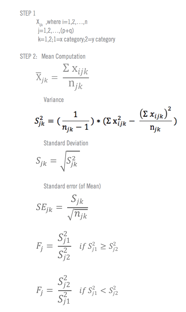
Related resources
Analysis & Reporting
Margin of error 11 min read
Data saturation in qualitative research 8 min read, thematic analysis 11 min read, behavioral analytics 12 min read, statistical significance calculator: tool & complete guide 18 min read, regression analysis 19 min read, data analysis 31 min read, request demo.
Ready to learn more about Qualtrics?

12 Chapter 12: Repeated Measures t-test
So far, we have dealt with data measured on a single variable at a single point in time, allowing us to gain an understanding of the logic and process behind statistics and hypothesis testing. Now, we will look at a slightly different type of data that has new information we couldn’t get at before: change. Specifically, we will look at how the value of a variable, within people , changes across two timepoints. This is a very powerful thing to do, and, as we will see shortly, it involves only a very slight addition to our existing process and does not change the mechanics of hypothesis testing or formulas at all!
Change and Differences
Researchers are often interested in change over time. Sometimes we want to see if change occurs naturally, and other times we are hoping for change in response to some manipulation. In each of these cases, we measure a single variable at different times, and what we are looking for is whether or not we get the same score at time 2 as we did at time 1. This is a repeated sample research design , where a single group of individuals is obtained and each individual is measured in two treatment conditions that are then compared. Data consist of two scores for each individual. This means that all subjects participate in each treatment condition. Think about it like a pretest/posttest.
When we analyze data for a repeated research design, we calculate the difference between members of each pair of scores and then take the average of those differences. The absolute value of our measurements does not matter – all that matters is the change. If the average difference between scores in our sample is very large, compared to the difference between scores we would expect if the member was selected from the same population then we will conclude that the individuals were selected from different populations.
Let’s look at an example:
| Before | After | Improvement |
| 6 | 9 | 3 |
| 7 | 7 | 0 |
| 4 | 10 | 6 |
| 1 | 3 | 2 |
| 8 | 10 | 2 |
Table 1. Raw and difference scores before and after training.
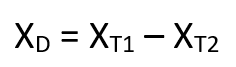
In both of these types of data, what we have are multiple scores on a single variable. That is, a single observation or data point is comprised of two measurements that are put together into one difference score. This is what makes the analysis of change unique – our ability to link these measurements in a meaningful way. This type of analysis would not work if we had two separate samples of people that weren’t related at the individual level, such as samples of people from different states that we gathered independently. Such datasets and analyses are the subject of the following chapter.
A rose by any other name…
It is important to point out that this form of t -test has been called many different things by many different people over the years: “matched pairs”, “paired samples”, “repeated measures”, “dependent measures”, “dependent samples”, and many others. What all of these names have in common is that they describe the analysis of two scores that are related in a systematic way within people or within pairs, which is what each of the datasets usable in this analysis have in common. As such, all of these names are equally appropriate, and the choice of which one to use comes down to preference. In this text, we will refer to paired samples , though the appearance of any of the other names throughout this chapter should not be taken to refer to a different analysis: they are all the same thing.

2 cups of tea for me: for a repeated measures design the same individuals are in both conditions for a t-test. Photo credit
Now that we have an understanding of what difference scores are and know how to calculate them, we can use them to test hypotheses. As we will see, this works exactly the same way as testing hypotheses about one sample mean with a t- statistic. The only difference is in the format of the null and alternative hypotheses, where for focus on the difference score.
Hypotheses of Change and Differences for step 1
When we work with difference scores, our research questions have to do with change. Did scores improve? Did symptoms get better? Did prevalence go up or down? Our hypotheses will reflect this. Remember that the null hypothesis is the idea that there is nothing interesting, notable, or impactful represented in our dataset. In a paired samples t-test, that takes the form of ‘no change’. There is no improvement in scores or decrease in symptoms.
Just as before, you choice of which alternative hypothesis to use should be specified before you collect data based on your research question and any evidence you might have that would indicate a specific directional (or non-directional) change. Additionally, it should be noted that a non-directional research/alternative hypothesis is a more conservative approach when you have an expected direction for change.
Choosing 1-tail vs 2-tail test
How do you choose whether to use a one-tailed versus a two-tailed test? The two-tailed test is always going to be more conservative, so it’s always a good bet to use that one, unless you had a very strong prior reason for using a one-tailed test. In that case, you should have written down the hypothesis before you ever looked at the data. In Chapter 19, we will discuss the idea of pre-registration of hypotheses, which formalizes the idea of writing down your hypotheses before you ever see the actual data. You should never make a decision about how to perform a hypothesis test once you have looked at the data, as this can introduce serious bias into the results.
We do have to make one main assumption when we use the randomization test, which we refer to as exchangeability . This means that all of the observations are distributed in the same way, such that we can interchange them without changing the overall distribution. The main place where this can break down is when there are related observations in the data; for example, if we had data from individuals in 4 different families, then we couldn’t assume that individuals were exchangeable, because siblings would be closer to each other than they are to individuals from other families. In general, if the data were obtained by random sampling, then the assumption of exchangeability should hold.
Critical Values and Decision Criteria for step 2
As with before, once we have our hypotheses laid out, we need to find our critical values that will serve as our decision criteria. This step has not changed at all from the last chapter. Our critical values are based on our level of significance (still usually α = 0.05), the directionality of our test (one-tailed or two-tailed), and the degrees of freedom, which are still calculated as df = n – 1. Because this is a t -test like the last chapter, we will find our critical values on the same t -table using the same process of identifying the correct column based on our significance level and directionality and the correct row based on our degrees of freedom or the next lowest value if our exact degrees of freedom are not presented. After we calculate our test statistic, our decision criteria are the same as well: p < α or t obt > t crit *.
Test Statistic for step 3
Our test statistic for our change scores follows exactly the same format as it did for our 1-sample t -test. In fact, the only difference is in the data that we use. For our change test, we first calculate a difference score as shown above. Then, we use those scores as the raw data in the same mean calculation, standard error formula, and t -statistic. Let’s look at each of these.
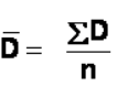
Here we are using the subscript D to keep track of that fact that these are difference scores instead of raw scores; it has no actual effect on our calculation.
Using this, we calculate the standard deviation of the difference scores the same way as well:
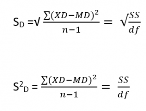
We will find the numerator, the Sum of Squares, using the same table format that we learned in chapter 3. Once we have our standard deviation, we can find the standard error:
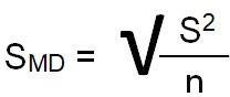
Finally, our test statistic t has the same structure as well:
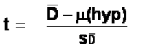
As we can see, once we calculate our difference scores from our raw measurements, everything else is exactly the same. Let’s see an example.
Example: Increasing Satisfaction at Work
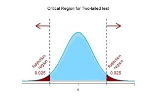
Hopefully the above example made it clear that running a dependent samples t -test to look for differences before and after some treatment works exactly the same way as a regular 1-sample t -test does from chapter 11 (which was just a small change in how z -tests were performed in chapter 10). At this point, this process should feel familiar, and we will continue to make small adjustments to this familiar process as we encounter new types of data to test new types of research questions.
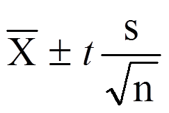
Example with Confidence Interval Hypothesis Testing: Bad Press
Let’s say that a bank wants to make sure that their new commercial will make them look good to the public, so they recruit 7 people to view the commercial as a focus group. The focus group members fill out a short questionnaire about how they view the company, then watch the commercial and fill out the same questionnaire a second time. The bank really wants to find significant results, so they test for a change at α = 0.05. However, they use a 2-tailed test since they know that past commercials have not gone over well with the public, and they want to make sure the new one does not backfire. They decide to test their hypothesis using a confidence interval to see just how spread out the opinions are. As we will see, confidence intervals work the same way as they did before, just like with the test statistic.
Step 1: State the Hypotheses
As always, we start with hypotheses, and with confidence interval hypothesis test, we must use a 2-tail test.
H 0 : There is no change in how people view the bank H 0 : μ D = 0
H A : There is a change in how people view the bank H A : μ D ≠ 0
Step 2: Find the Critical Values
Just like with our regular hypothesis testing procedure, we will need critical values from the appropriate level of significance and degrees of freedom in order to form our confidence interval. Because we have 7 participants, our degrees of freedom are df = 6. From our t -table, we find that the critical value corresponding to this df at this level of significance is t * = 2.447.
Step 3: Calculate the Confidence Interval
The data collected before (time 1) and after (time 2) the participants viewed the commercial is presented in Table 1. In order to build our confidence interval, we will first have to calculate the mean and standard deviation of the difference scores, which are also in Table 1. As a reminder, the difference scores ( D̅ or M D ) are calculated as Time 2 – Time 1.
| Time 1 | Time 2 | D̅ |
| 3 | 2 | -1 |
| 3 | 6 | 3 |
| 5 | 3 | -2 |
| 8 | 4 | -4 |
| 3 | 9 | 6 |
| 1 | 2 | 1 |
| 4 | 5 | 1 |
Table 1. Opinions of the bank
The mean of the difference scores is: D̅ = 4/7 = .57
The standard deviation will be solved by first using the Sum of Squares Table:
| D | D –D̅ | (D –D̅) |
| -1 | -1.57 | 2.46 |
| 3 | 2.43 | 5.90 |
| -2 | -2.57 | 6.60 |
| -4 | -4.57 | 20.88 |
| 6 | 5.43 | 29.48 |
| 1 | 0.43 | 0.18 |
| 1 | 0.43 | 0.18 |
| Σ = 4 | Σ = 0 | Σ = 65.68 (our SS) |
s = √SS/df where SS = 65.68 and df = n-1 = 7-1 = 6
Step 4: Make the Decision
Remember that the confidence interval represents a range of values that seem plausible or reasonable based on our observed data. The interval spans -1.86 to 3.00, which includes 0, our null hypothesis value. Because the null hypothesis value is in the interval, it is considered a reasonable value, and because it is a reasonable value, we have no evidence against it. We fail to reject the null hypothesis.
Assumptions are conditions that must be met in order for our hypothesis testing conclusion to be valid. [Important: If the assumptions are not met then our hypothesis testing conclusion is not likely to be valid. Testing errors can still occur even if the assumptions for the test are met.]
Recall that inferential statistics allow us to make inferences (decisions, estimates, predictions) about a population based on data collected from a sample. Recall also that an inference about a population is true only if the sample studied is representative of the population. A statement about a population based on a biased sample is not likely to be true.
Assumption 1 : Individuals in the sample were selected randomly and independently, so the sample is highly likely to be representative of the larger population.
• Random sampling ensures that each member of the population is equally likely to be selected.
• An independent sample is one which the selection of one member has no effect on the selection of any other.
Assumption 2: The distribution of sample differences (DSD) is a normal, because we drew the samples from a population that was normally distributed.
- This assumption is very important because we are estimating probabilities using the t- table – which provide accurate estimates of probabilities for events distributed normally.
Assumption 3: Sampled populations have equal variances or have homogeneity of variance.
Advantages & Disadvantages of using a repeated measures design
Advantages. Repeated measure designs reduce the probability of Type I errors when compared with independent sample designs because repeated measure t-tests reduce the probability that we will get a statistically significant difference that is due to an extraneous variable that differed between groups by chance (due to some other factor than the one in which we are interested).
Repeated measure designs are also more powerful (sensitive) than independent sample designs because two scores from each person are compared so each person serves as his or her own control group (we analyze the difference between scores). A special type of repeated measures design is known as the matched pairs design. If we are designing a study and suspect that there are important factors that could differ between our groups even if we randomly select and assign subjects, then we may use this type of design.
Because members of a matched-pair are similar to each other there is greater likelihood of our statistical test finding an “effect” when one person is present (power) in a repeated sample design as compared to a two-repeated sample design (in which subjects for two groups are picked randomly and independently – not matched on any traits).
Disadvantages. Repeated measure t-tests are very sensitive to outside influences and treatment influences. Outside Influences refers to factors outside of the experiment that may interfere with testing an individual across treatment/trials. Examples include mood or health or motivation of the individual participants. Think about it, if a participant tries really hard during the pretest but does not try very hard during the posttest, these differences can create problems later when analyzing the data.
Treatment Influences refers to the events that happen within the testing experience that interferes with how the data are collected. Three of the most common treatment influences are: 1. Practice effects, 2. Fatigue effects, and 3. Order effects.
Practice effect is present where participants perform a task better in later conditions because they have had a chance to practice it. Another type is a fatigue effect, where participants perform a task worse in later conditions because they become tired or bored. Order effects refer to differences in research participants’ responses that result from the order (e.g., first, second, third) in which the experimental materials are presented to them.
Imagine, for example, that participants judge the guilt of an attractive defendant and then judge the guilt of an unattractive defendant. If they judge the unattractive defendant more harshly, this might be because of his unattractiveness. But it could be instead that they judge him more harshly because they are becoming bored or tired. In other words, the order of the conditions is a confounding variable. The attractive condition is always the first condition and the unattractive condition the second. Thus any difference between the conditions in terms of the dependent variable could be caused by the order of the conditions and not the independent variable itself.
There is a solution to the problem of order effects, however, that can be used in many situations. It is counterbalancing, which means testing different participants in different orders. For example, some participants would be tested in the attractive defendant condition followed by the unattractive defendant condition, and others would be tested in the unattractive condition followed by the attractive condition. With three conditions, there would be six different orders (ABC, ACB, BAC, BCA, CAB, and CBA), so some participants would be tested in each of the six orders. With counterbalancing, participants are assigned to orders randomly, using the techniques we have already discussed. Thus random assignment plays an important role in within-subjects designs just as in between-subjects designs. Here, instead of randomly assigning to conditions, they are randomly assigned to different orders of conditions. In fact, it can safely be said that if a study does not involve random assignment in one form or another, it is not an experiment.
Because the repeated-measures design requires that each individual participate in more than one treatment, there is always the risk that exposure to the first treatment will cause a change in the participants that influences their scores in the second treatment that have nothing to do with the intervention. For example, if students are given the same test before and after the intervention the change in the posttest might be because the student got practice taking the test, not because the intervention was successful.
Learning Objectives
Having read this chapter, a student should be able to:
- identify when appropriate to calculate a paired or dependent t-test
- perform a hypothesis test using the paired or dependent t-test
- compute and interpret effect size for dependent or paired t-test
- list the assumptions for running a paired or dependent t-test
- list the advantages and disadvantages for a repeated measures design
Exercises – Ch. 12
- What is the difference between a 1-sample t -test and a dependent-samples t – test? How are they alike?
- Name 3 research questions that could be addressed using a dependent- samples t -test.
- What are difference scores and why do we calculate them?
- Why is the null hypothesis for a dependent-samples t -test always μ D = 0?
- A researcher is interested in testing whether explaining the processes of statistics helps increase trust in computer algorithms. He wants to test for a difference at the α = 0.05 level and knows that some people may trust the algorithms less after the training, so he uses a two-tailed test. He gathers pre- post data from 35 people and finds that the average difference score is 12.10 with a standard deviation (s) is 17.39. Conduct a hypothesis test to answer the research question.
- M𝐷̅ = 3.50, s = 1.10, n = 12, α = 0.05, two-tailed test
- 95% CI = (0.20, 1.85)
- t = 2.98, t * = -2.36, one-tailed test to the left
- 90% CI = (-1.12, 4.36)
- Calculate difference scores for the following data:
| Time 1 | Time 2 | X or D |
| 61 | 83 |
|
| 75 | 89 |
|
| 91 | 98 |
|
| 83 | 92 |
|
| 74 | 80 |
|
| 82 | 88 |
|
| 98 | 98 |
|
| 82 | 77 |
|
| 69 | 88 |
|
| 76 | 79 |
|
| 91 | 91 |
|
| 70 | 80 |
|
8. You want to know if an employee’s opinion about an organization is the same as the opinion of that employee’s boss. You collect data from 18 employee-supervisor pairs and code the difference scores so that positive scores indicate that the employee has a higher opinion and negative scores indicate that the boss has a higher opinion (meaning that difference scores of 0 indicate no difference and complete agreement). You find that the mean difference score is ̅𝑋̅̅𝐷̅ = -3.15 with a standard deviation of s D = 1.97. Test this hypothesis at the α = 0.01 level.
9. Construct confidence intervals from a mean = 1.25, standard error of 0.45, and d f = 10 at the 90%, 95%, and 99% confidence level. Describe what happens as confidence changes and whether to reject H 0 .
10.A professor wants to see how much students learn over the course of a semester. A pre-test is given before the class begins to see what students know ahead of time, and the same test is given at the end of the semester to see what students know at the end. The data are below. Test for an improvement at the α = 0.05 level. Did scores increase? How much did scores increase?
| Pretest | Posttest | X |
| 90 | 8 |
|
| 60 | 66 |
|
| 95 | 99 |
|
| 93 | 91 |
|
| 95 | 100 |
|
| 67 | 64 |
|
| 89 | 91 |
|
| 90 | 95 |
|
| 94 | 95 |
|
| 83 | 89 |
|
| 75 | 82 |
|
| 87 | 92 |
|
| 82 | 83 |
|
| 82 | 85 |
|
| 88 | 93 |
|
| 66 | 69 |
|
| 90 | 90 |
|
| 93 | 100 |
|
| 86 | 95 |
|
| 91 | 96 |
|
Answers to Odd- Numbered Exercises – Ch. 12
1. A 1-sample t -test uses raw scores to compare an average to a specific value. A dependent samples t -test uses two raw scores from each person to calculate difference scores and test for an average difference score that is equal to zero. The calculations, steps, and interpretation is exactly the same for each.
7. See table last column.
| Time 1 | Time 2 | D or X |
| 61 | 83 | 22 |
| 75 | 89 | 14 |
| 91 | 98 | 7 |
| 83 | 92 | 9 |
| 74 | 80 | 6 |
| 82 | 88 | 6 |
| 98 | 98 | 0 |
| 82 | 77 | -5 |
| 69 | 88 | 19 |
| 76 | 79 | 3 |
| 91 | 91 | 0 |
| 70 | 80 | 10 |
9. At the 90% confidence level, t * = 1.812 and CI = (0.43, 2.07) so we reject H 0 . At the 95% confidence level, t * = 2.228 and CI = (0.25, 2.25) so we reject H 0 . At the 99% confidence level, t * = 3.169 and CI = (-0.18, 2.68) so we fail to reject H 0 . As the confidence level goes up, our interval gets wider (which is why we have higher confidence), and eventually we do not reject the null hypothesis because the interval is so wide that it contains 0.
Introduction to Statistics for Psychology Copyright © 2021 by Alisa Beyer is licensed under a Creative Commons Attribution-NonCommercial-ShareAlike 4.0 International License , except where otherwise noted.
Share This Book
Dependent t-test for paired samples
What does this test do.
The dependent t-test (also called the paired t-test or paired-samples t-test) compares the means of two related groups to determine whether there is a statistically significant difference between these means.
What variables do you need for a dependent t-test?
You need one dependent variable that is measured on an interval or ratio scale (see our Types of Variable guide if you need clarification). You also need one categorical variable that has only two related groups.
What is meant by "related groups"?
A dependent t-test is an example of a "within-subjects" or "repeated-measures" statistical test. This indicates that the same participants are tested more than once. Thus, in the dependent t-test, "related groups" indicates that the same participants are present in both groups. The reason that it is possible to have the same participants in each group is because each participant has been measured on two occasions on the same dependent variable. For example, you might have measured the performance of 10 participants in a spelling test (the dependent variable) before and after they underwent a new form of computerised teaching method to improve spelling. You would like to know if the computer training improved their spelling performance. Here, we can use a dependent t-test because we have two related groups. The first related group consists of the participants at the beginning (prior to) the computerised spell training and the second related group consists of the same participants, but now at the end of the computerised training.

Does the dependent t-test test for "changes" or "differences" between related groups?
The dependent t-test can be used to test either a "change" or a "difference" in means between two related groups, but not both at the same time. Whether you are measuring a "change" or "difference" between the means of the two related groups depends on your study design. The two types of study design are indicated in the following diagrams.
How do you detect differences between experimental conditions using the dependent t-test?
The dependent t-test can look for "differences" between means when participants are measured on the same dependent variable under two different conditions. For example, you might have tested participants' eyesight (dependent variable) when wearing two different types of spectacle (independent variable). See the diagram below for a general schematic of this design approach (click the image to enlarge):

Find out more about the dependent t-test on the next page .
- Skip to secondary menu
- Skip to main content
- Skip to primary sidebar
Statistics By Jim
Making statistics intuitive
How t-Tests Work: 1-sample, 2-sample, and Paired t-Tests
By Jim Frost 15 Comments
T-tests are statistical hypothesis tests that analyze one or two sample means. When you analyze your data with any t-test, the procedure reduces your entire sample to a single value, the t-value. In this post, I describe how each type of t-test calculates the t-value. I don’t explain this just so you can understand the calculation, but I describe it in a way that really helps you grasp how t-tests work.

How 1-Sample t-Tests Calculate t-Values
The equation for how the 1-sample t-test produces a t-value based on your sample is below:

This equation is a ratio, and a common analogy is the signal-to-noise ratio. The numerator is the signal in your sample data, and the denominator is the noise. Let’s see how t-tests work by comparing the signal to the noise!
The Signal – The Size of the Sample Effect
In the signal-to-noise analogy, the numerator of the ratio is the signal. The effect that is present in the sample is the signal. It’s a simple calculation. In a 1-sample t-test, the sample effect is the sample mean minus the value of the null hypothesis. That’s the top part of the equation.
For example, if the sample mean is 20 and the null value is 5, the sample effect size is 15. We’re calling this the signal because this sample estimate is our best estimate of the population effect.
The calculation for the signal portion of t-values is such that when the sample effect equals zero, the numerator equals zero, which in turn means the t-value itself equals zero. The estimated sample effect (signal) equals zero when there is no difference between the sample mean and the null hypothesis value. For example, if the sample mean is 5 and the null value is 5, the signal equals zero (5 – 5 = 0).
The size of the signal increases when the difference between the sample mean and null value increases. The difference can be either negative or positive, depending on whether the sample mean is greater than or less than the value associated with the null hypothesis.
A relatively large signal in the numerator produces t-values that are further away from zero.

The Noise – The Variability or Random Error in the Sample
The denominator of the ratio is the standard error of the mean, which measures the sample variation. The standard error of the mean represents how much random error is in the sample and how well the sample estimates the population mean.
As the value of this statistic increases, the sample mean provides a less precise estimate of the population mean. In other words, high levels of random error increase the probability that your sample mean is further away from the population mean.
In our analogy, random error represents noise. Why? When there is more random error, you are more likely to see considerable differences between the sample mean and the null hypothesis value in cases where the null is true . Noise appears in the denominator to provide a benchmark for how large the signal must be to distinguish from the noise.
Signal-to-Noise ratio
Our signal-to-noise ratio analogy equates to:

Both of these statistics are in the same units as your data. Let’s calculate a couple of t-values to see how to interpret them.
- If the signal is 10 and the noise is 2, your t-value is 5. The signal is 5 times the noise.
- If the signal is 10 and the noise is 5, your t-value is 2. The signal is 2 times the noise.
The signal is the same in both examples, but it is easier to distinguish from the lower amount of noise in the first example. In this manner, t-values indicate how clear the signal is from the noise. If the signal is of the same general magnitude as the noise, it’s probable that random error causes the difference between the sample mean and null value rather than an actual population effect.
Paired t-Tests Are Really 1-Sample t-Tests
Paired t-tests require dependent samples. I’ve seen a lot of confusion over how a paired t-test works and when you should use it. Pssst! Here’s a secret! Paired t-tests and 1-sample t-tests are the same hypothesis test incognito!
You use a 1-sample t-test to assess the difference between a sample mean and the value of the null hypothesis.
A paired t-test takes paired observations (like before and after), subtracts one from the other, and conducts a 1-sample t-test on the differences. Typically, a paired t-test determines whether the paired differences are significantly different from zero.
Download the CSV data file to check this yourself: T-testData . All of the statistical results are the same when you perform a paired t-test using the Before and After columns versus performing a 1-sample t-test on the Differences column.

Once you realize that paired t-tests are the same as 1-sample t-tests on paired differences, you can focus on the deciding characteristic —does it make sense to analyze the differences between two columns?
Suppose the Before and After columns contain test scores and there was an intervention in between. If each row in the data contains the same subject in the Before and After column, it makes sense to find the difference between the columns because it represents how much each subject changed after the intervention. The paired t-test is a good choice.
On the other hand, if a row has different subjects in the Before and After columns, it doesn’t make sense to subtract the columns. You should use the 2-sample t-test described below.
The paired t-test is a convenience for you. It eliminates the need for you to calculate the difference between two columns yourself. Remember, double-check that this difference is meaningful! If using a paired t-test is valid, you should use it because it provides more statistical power than the 2-sample t-test, which I discuss in my post about independent and dependent samples .
How Two-Sample T-tests Calculate T-Values
Use the 2-sample t-test when you want to analyze the difference between the means of two independent samples. This test is also known as the independent samples t-test . Click the link to learn more about its hypotheses, assumptions, and interpretations.
Like the other t-tests, this procedure reduces all of your data to a single t-value in a process similar to the 1-sample t-test. The signal-to-noise analogy still applies.
Here’s the equation for the t-value in a 2-sample t-test.

The equation is still a ratio, and the numerator still represents the signal. For a 2-sample t-test, the signal, or effect, is the difference between the two sample means. This calculation is straightforward. If the first sample mean is 20 and the second mean is 15, the effect is 5.
Typically, the null hypothesis states that there is no difference between the two samples. In the equation, if both groups have the same mean, the numerator, and the ratio as a whole, equals zero. Larger differences between the sample means produce stronger signals.
The denominator again represents the noise for a 2-sample t-test. However, you can use two different values depending on whether you assume that the variation in the two groups is equal or not. Most statistical software let you choose which value to use.
Regardless of the denominator value you use, the 2-sample t-test works by determining how distinguishable the signal is from the noise. To ascertain that the difference between means is statistically significant, you need a high positive or negative t-value.
How Do T-tests Use T-values to Determine Statistical Significance?
Here’s what we’ve learned about the t-values for the 1-sample t-test, paired t-test, and 2-sample t-test:
- Each test reduces your sample data down to a single t-value based on the ratio of the effect size to the variability in your sample.
- A t-value of zero indicates that your sample results match the null hypothesis precisely.
- Larger absolute t-values represent stronger signals, or effects, that stand out more from the noise.
For example, a t-value of 2 indicates that the signal is twice the magnitude of the noise.
Great … but how do you get from that to determining whether the effect size is statistically significant? After all, the purpose of t-tests is to assess hypotheses. To find out, read the companion post to this one: How t-Tests Work: t-Values, t-Distributions and Probabilities . Click here for step-by-step instructions on how to do t-tests in Excel !
If you’d like to learn about other hypothesis tests using the same general approach, read my posts about:
- How F-tests Work in ANOVA
- How Chi-Squared Tests of Independence Work
Share this:

Reader Interactions

January 9, 2023 at 11:11 am
Hi Jim, thank you for explaining this I will revert to this during my 8 weeks in class everyday to make sure I understand what I’m doing . May I ask more questions in the future.

November 27, 2021 at 1:37 pm
This was an awesome piece, very educative and easy to understand

June 19, 2021 at 1:53 pm
Hi Jim, I found your posts very helpful. Could you plz explain how to do T test for a panel data?

June 19, 2021 at 3:40 pm
You’re limited by what you can do with t-tests. For panel data and t-tests, you can compare the same subjects at two points in time using a paired t-test. For more complex arrangements, you can use repeated measures ANOVA or specify a regression model to meet your needs.

February 11, 2020 at 10:34 pm
Hi Jim: I was reviewing this post in preparation for an analysis I plan to do, and I’d like to ask your advice. Each year, staff complete an all-employee survey, and results are reported at workgroup level of analysis. I would like to compare mean scores of several workgroups from one year to the next (in this case, 2018 and 2019 scores). For example, I would compare workgroup mean scores on psychological safety between 2018 and 2019. I am leaning toward a paired t test. However, my one concern is that….even though I am comparing workgroup to workgroup from one year to the next….it is certainly possible that there may be some different employees in a given workgroup from one year to the next (turnover, transition, etc.)….Assuming that is the case with at least some of the workgroups, does that make a paired t test less meanginful? Would I still use a paired t test or would another type t test be more appropriate? I’m thinking because we are dealing with workgroup mean scores (and not individual scores), then it may still be okay to compare meaningfully (avoiding an ecological fallacy). Thoughts?
Many thanks for these great posts. I enjoy reading them…!

April 8, 2019 at 11:22 pm
Hi jim. First of all, I really appreciate your posts!
When I use t-test via R or scikit learn, there is an option for homogeneity of variance. I think that option only applied to two sample t-test, but what should I do for that option?
Should I always perform f-test for check the homogeneity of variance? or Which one is a more strict assumption?

November 9, 2018 at 12:03 am
This blog is great. I’m at Stanford and can say this is a great supplement to class lectures. I love the fact that there aren’t formulas so as to get an intuitive feel. Thank you so much!
November 9, 2018 at 9:12 am
Thanks Mel! I’m glad it has been helpful! Your kind words mean a lot to me because I really strive to make these topics as easy to understand as possible!

December 29, 2017 at 4:14 pm
Thank you so much Jim! I have such a hard time understanding statistics without people like you who explain it using words to help me conceptualize rather than utilizing symbols only!
December 29, 2017 at 4:56 pm
Thank you, Jessica! Your kind words made my day. That’s what I want my blog to be all about. Providing simple but 100% accurate explanations for statistical concepts!
Happy New Year!

October 22, 2017 at 2:38 pm
Hi Jim, sure, I’ll go through it…Thank you..!
October 22, 2017 at 4:50 am
In summary, the t test tells, how the sample mean is different from null hypothesis, i.e. how the sample mean is different from null, but how does it comment about the significance? Is it like “more far from null is the more significant”? If it is so, could you give some more explanation about it?
October 22, 2017 at 2:30 pm
Hi Omkar, you’re in luck, I’ve written an entire blog post that talks about how t-tests actually use the t-values to determine statistical significance. In general, the further away from zero, the more significant it is. For all the information, read this post: How t-Tests Work: t-Values, t-Distributions, and Probabilities . I think this post will answer your questions.

September 12, 2017 at 2:46 am
Excellent explanation, appreciate you..!!
September 12, 2017 at 8:48 am
Thank you, Santhosh! I’m glad you found it helpful!
Comments and Questions Cancel reply
De-mystifying the Influence of PhET Simulation on Engagement, Satisfaction, and Academic Achievement of Bhutanese Students in the Physics Classroom
- Published: 26 June 2024
Cite this article

- Tshering Dorji ORCID: orcid.org/0000-0002-0022-6507 1 ,
- Sumitra Subba ORCID: orcid.org/0009-0006-4783-5752 1 &
- Tshering Zangmo ORCID: orcid.org/0009-0003-9253-7314 2
This study employed a non-equivalent quasi-experimental pre-test/post-test control-group design to study the effect of the PhET simulation intervention on students’ engagement, satisfaction, and academic achievement in the learning of direct current electric circuit concepts among Bhutanese students. We analysed the pre- and post-test scores and perceptions of 57 ninth-grade students, divided into experimental group (EG, n = 29) and control group (CG, n = 28), from one high school in Paro District, Bhutan . The EG students were taught with the PhET simulation intervention, while the CG students were taught with the traditional chalk-talk method. The pre- and post-test scores were collected with the Electric Circuits Conceptual Evaluation (ECEE) inventory. Mean, standard deviation, a two-sample t -test, and multiple linear regression (MLR) were computed using R and RStudio. The t -test revealed a statistically significant difference in the mean post-test scores of CG and EG students. MLR analysis further confirmed that this difference was due to the PhET simulation intervention, ruling out the influence of other confounding variables. Additionally, an instrument called the PhET Engagement-Satisfaction Questionnaire was developed to assess EG students’ engagement level and satisfaction with the PhET simulation intervention. Confirmatory factor analysis and Cronbach’s alpha calculation confirmed its validity and reliability. Data from the PhET Engagement-Satisfaction Questionnaire unveiled significant impact of the PhET simulation intervention on students’ engagement level and their overall satisfaction, reinforcing prior research. However, further research with a larger sample size, incorporating lesson observations, interviews, and our measurement tool, is necessary to ascertain whether the findings it yields align with the present study’s findings.
This is a preview of subscription content, log in via an institution to check access.
Access this article
Price includes VAT (Russian Federation)
Instant access to the full article PDF.
Rent this article via DeepDyve
Institutional subscriptions
Availability of Data and Materials
The R code and raw datasets used and/or analysed during the current study are available from the corresponding author on request.
Alhadlaq, A. (2023). Computer-based simulated learning activities: Exploring Saudi students’ attitude and experience of using simulations to facilitate unsupervised learning of science concepts. Applied Sciences, 13 (7), 4583. https://doi.org/10.3390/app13074583
Article Google Scholar
Almasri, F. (2022). Simulations to teach science subjects: Connections among students’ engagement, self-confidence, satisfaction, and learning styles. Education and Information Technologies, 27 (5), 7161–7181. https://doi.org/10.1007/s10639-022-10940-w
Andrade, C. (2021). The inconvenient truth about convenience and purposive samples. Indian Journal of Psychological Medicine, 43 (1), 86–88. https://doi.org/10.1177/0253717620977000
Babin, M. J., Riviere, E., & Chiniara, G. (2019). Theory for practice: Learning theories for simulation. In G. Chiniara (Ed.), Clinical simulation (2nd ed., pp. 97–114). Academic Press. https://doi.org/10.1016/B978-0-12-815657-5.00008-5
Chapter Google Scholar
Banda, H. J., & Nzabahimana, J. (2021). Effect of integrating physics education technology simulations on students’ conceptual understanding in physics: A review of literature. Physical Review Physics Education Research, 17 (2), 023108. https://doi.org/10.1103/PhysRevPhysEducRes.17.023108
Banda, H. J., & Nzabahimana, J. (2022). The impact of physics education technology (PhET) interactive simulation-based learning on motivation and academic achievement among Malawian physics students. Journal of Science Education and Technology, 32 , 127–141. https://doi.org/10.1007/s10956-022-10010-3
Bo, W. V., Fulmer, G. W., Lee, C. K. E., & Chen, V. D. T. (2018). How do secondary science teachers perceive the use of interactive simulations? The affordance in Singapore context. Journal of Science Education and Technology, 27 , 550–565. https://doi.org/10.1007/s10956-018-9744-2
Chatterjee, S., & Hadi, A. S. (2013). Regression analysis by example . John Wiley & Sons.
Google Scholar
Childs, A., Tenzin, W., Johnson, D., & Ramachandran, K. (2012). Science education in Bhutan: Issues and challenges. International Journal of Science Education, 34 (3), 375–400. https://doi.org/10.1080/09500693.2011.626461
Chinaka, T. W. (2021). The effect of PhET simulation vs. phenomenon-based experiential learning on students’ integration of motion along two independent axes in projectile motion. African Journal of Research in Mathematics, Science and Technology Education, 25 (2), 185–196.
Cohen, J. (1992). A power primer. Psychological Bulletin, 112 , 155–159. https://doi.org/10.1037/0033-2909.112.1.155
Cronk, B. C. (2020). How to use SPSS: A step-by-step guide to analysis and interpretation (11th ed.). Routledge. https://doi.org/10.4324/9780429340321
Book Google Scholar
Davis, F. D. (1987). Technology acceptance model: TAM. Al-Suqri, MN, Al-Aufi, AS: Information Seeking Behavior and Technology Adoption, 205 , 219. https://quod.lib.umich.edu/b/busadwp/images/b/1/4/b1409190.0001.001.pdf
Demetriou, C., Ozer, B. U., & Essau, C. A. (2015). Self-report questionnaires. In R. L. Cautin & S. O. Lilienfeld (Eds.), The encyclopedia of clinical psychology (pp. 1–6). Wiley. https://doi.org/10.1002/9781118625392.wbecp507
Dendup, P. (2023). English medium instruction in the Bhutanese education system: A historical journey. In R. A. Giri, A. Padwad, & M. M. N. Kabir (Eds.), English as a medium of instruction in South Asia (pp. 145–155). Routledge. https://doi.org/10.4324/9781003342373
Doll, W. J., Raghunathan, T. S., Lim, J. S., & Gupta, Y. P. (1995). A confirmatory factor analysis of the user information satisfaction instrument. Information Systems Research, 6 (2), 177–188. https://doi.org/10.1287/isre.6.2.177
Faber, J., & Fonseca, L. M. (2014). How sample size influences research outcomes. Dental Press Journal of Orthodontics, 19 (4), 27–29. https://doi.org/10.1590/2176-9451.19.4.027-029.ebo
Falloon, G. (2019). Using simulations to teach young students science concepts: An experiential learning theoretical analysis. Computers & Education, 135 , 138–159. https://doi.org/10.1016/j.compedu.2019.03.001
Fussell, S. G., & Truong, D. (2022). Using virtual reality for dynamic learning: An extended technology acceptance model. Virtual Reality, 26 (1), 249–267. https://doi.org/10.1007/s10055-021-00554-x
Ganasen, S., & Shamuganathan, S. (2017). The effectiveness of physics education technology (PhET) interactive simulations in enhancing matriculation students’ understanding of chemical equilibrium and remediating their misconceptions. Overcoming students’ misconceptions in science: Strategies and perspectives from Malaysia (pp. 157–178). Springer.
Gani, A., Syukri, M., Khairunnisak, K., Nazar, M., Sari, R. P., Nazar, N., Sari, R. P., Nazar, M., & Sari, R. P. (2020). Improving concept understanding and motivation of learners through Phet simulation word. Journal of Physics: Conference Series, 1567 , 042013. https://doi.org/10.1088/1742-6596/1567/4/042013
George, D., & Mallery, P. (2019). IBM SPSS statistics 26 step by step: A simple guide and reference (16th ed.). Routledge.
Haryadi, R., & Pujiastuti, H. (2020). PhET simulation software-based learning to improve science process skills. Journal of Physics: Conference Series, 1521 (2), 022017. https://doi.org/10.1088/1742-6596/1521/2/022017 . IOP Publishing.
Hu, L. T., & Bentler, P. M. (1999). Cutoff criteria for fit indexes in covariance structure analysis: Conventional criteria versus new alternatives. Structural Equation Modeling: A Multidisciplinary Journal, 6 (1), 1–55. https://doi.org/10.1080/10705519909540118
Jeffries, P. R., & Rizzolo, M. A. (2006). Designing and implementing models for the innovative use of using simulation to teach nursing care of Ill adults and children: A national, multi-site, multi-method study . National League for Nursing.
Kallner, A. (2018). Formulas. In A. Kallner (Ed.), Laboratory statistics: Methods in chemistry and health science (2nd ed., pp. 1–140). Elsevier. https://doi.org/10.1016/C2017-0-00959-X
Kinley, Rai, R., & Chophel, S. (2021). A journey towards STEM education in Bhutan: An educational review. In T. W. Teo, A. Tan, & P. Teng (Eds.), STEM education from Asia: Trends and perspectives (pp. 49–62). Routledge. https://doi.org/10.4324/9781003099888
Kolb, D. A. (2014). Experiential learning: Experience as the source of learning and development (2nd ed.). Pearson Education Inc.
Lebowitz, E. R., Marin, C. E., & Silverman, W. K. (2019). Measuring family accommodation of childhood anxiety: Confirmatory factor analysis, validity, and reliability of the parent and child family accommodation scale–anxiety. Journal of Clinical Child & Adolescent Psychology . https://doi.org/10.1080/15374416.2019.1614002
Lee, W. C., Neo, W. L., Chen, D. T., & Lin, T. B. (2021). Fostering changes in teacher attitudes toward the use of computer simulations: Flexibility, pedagogy, usability and needs. Education and Information Technologies, 26 , 4905–4923. https://doi.org/10.1007/s10639-021-10506-2
Lehane, L. (2020). Experiential learning - David A. Kolb: Learning through experience. In B. Akpan & T. J. Kennedy (Eds.), Science education in theory and theory (pp. 241–257). Springer International Publishing. https://doi.org/10.1007/978-3-030-43620-9
Lei, M., & Lomax, R. G. (2005). The effect of varying degrees of nonnormality in structural equation modeling. Structural Equation Modeling, 12 (1), 1–27. https://doi.org/10.1207/s15328007sem1201_1
Li, C. H. (2016). Confirmatory factor analysis with ordinal data: Comparing robust maximum likelihood and diagonally weighted least squares. Behavior Research Methods, 48 , 936–949. https://doi.org/10.3758/s13428-015-0619-7
Lindgren, R., Tscholl, M., Wang, S., & Johnson, E. (2016). Enhancing learning and engagement through embodied interaction within a mixed reality simulation. Computers & Education, 95 , 174–187. https://doi.org/10.1016/j.compedu.2016.01.001
Liu, T. C., & Lin, Y. C. (2010). The application of Simulation-Assisted Learning Statistics (SALS) for correcting misconceptions and improving understanding of correlation. Journal of Computer Assisted Learning, 26 (2), 143–158.
Marsh, H. W., & Hocevar, D. (1985). Application of confirmatory factor analysis to the study of self-concept: First-and higher order factor models and their invariance across groups. Psychological bulletin, 97 (3), 562. https://doi.org/10.1037/0033-2909.97.3.562
Meyer, E. G., Battista, A., Sommerfeldt, J. M., West, J. C., Hamaoka, D., & Cozza, K. L. (2021). Experiential learning cycles as an effective means for teaching psychiatric clinical skills via repeated simulation in the psychiatry clerkship. Academic Psychiatry, 45 , 150–158. https://doi.org/10.1007/s40596-020-01340-8
Mishra, P., Pandey, C. M., Singh, U., Gupta, A., Sahu, C., & Keshri, A. (2019). Descriptive statistics and normality tests for statistical data. Annals of Cardiac Anaesthesia, 22 (1), 67–72. https://doi.org/10.4103/aca.aca_157_18
Mrani, C. A., El Hajjami, A., & El Khattabi, K. (2020). Effects of the integration of PhET simulations in the teaching and learning of the physical sciences of common core (Morocco). Universal Journal of Educational Research, 8 (7), 3014–3025. https://doi.org/10.13189/ujer.2020.080730
Penjor, T., Utha, K., & Seden, K. (2022). Effectiveness of simulation in teaching geometrical optics. International Journal of English Literature and Social Sciences, 7 (5), 88–94.
Perkins, K. (2020). Transforming STEM learning at scale: PhET interactive simulations. Childhood Education, 96 (4), 42–49. https://doi.org/10.1080/00094056.2020.1796451
Perkins, K., Moore, E., Podolefsky, N., Lancaster, K., & Denison, C. (2012). Towards research-based strategies for using PhET simulations in middle school physical science classes. In AIP Conference Proceedings, 1413 (1), 295–298. American Institute of Physics.
Petrus, R. M. (2015). Comparing the performance of national curriculum statements and old curriculum students’ in electric circuits. International Journal of Educational Sciences, 8 (3), 453–460. https://doi.org/10.1080/09751122.2015.11890267
Poore, J. A., Cullen, D. L., & Schaar, G. L. (2014). Simulation-based interprofessional education guided by Kolb’s experiential learning theory. Clinical Simulation in Nursing, 10 (5), e241–e247. https://doi.org/10.1016/j.ecns.2014.01.004
Pourhoseingholi, M. A., Baghestani, A. R., & Vahedi, M. (2012). How to control confounding effects by statistical analysis. Gastroenterology and Hepatology from Bed to Bench, 5 (2), 79. https://www.ncbi.nlm.nih.gov/pmc/articles/PMC4017459/
Prima, E. C., Putri, A. R., & Rustaman, N. (2018). Learning solar system using PhET simulation to improve students’ understanding and motivation. Journal of Science Learning, 1 (2), 60–70. https://doi.org/10.17509/jsl.v1i2.10239
Rehn, D. A., Moore, E. B., Podolefsky, N. S., & Finkelstein, N. D. (2013). Tools for high-tech tool use: A framework and heuristics for using interactive simulations. Journal of Teaching and Learning with Technology, 2 , 31–55. https://scholarworks.iu.edu/journals/index.php/jotlt/article/view/3507
Richardson, V. (2003). Constructivist pedagogy. Teachers College Record: THe Voice of Scholarship in Education, 105 (9), 1623–1640. https://doi.org/10.1046/j.1467-9620.2003.00303.x
Rodriguez-Segura, D. (2022). EdTech in developing countries: A review of the evidence. The World Bank Research Observer, 37 (2), 171–203. https://doi.org/10.1093/wbro/lkab011
Ross, J. M., & Bauldry, S. (2022). Confirmatory factor analysis: Quantitative applications in the social sciences (Vol. 189). SAGE Publications. Inc. https://us.sagepub.com/en-us/nam/confirmatory-factor-analysis/book269092#preview
Ross, S. M., Morrisson, G. R., & Lowther, D. L. (2010). Educational technology research past and present: Balancing rigor and relevance to impact school learning. Contemporary Educational Technology, 1 (1), 17–35.
Rosseel, Y. (2012). lavaan: An R package for structural equation modeling. Journal of Statistical Software, 48 (2), 1–36. https://doi.org/10.18637/jss.v048.i02
Rutten, N., Van Joolingen, W. R., & Van Der Veen, J. T. (2012). The learning effects of computer simulations in science education. Computers & Education, 58 (1), 136–153. https://doi.org/10.1016/j.compedu.2011.07.017
Ruwiyah, S., Rahman, N. F. A., Rahim, A. A., Yusof, M. Y., & Umar, S. H. (2021). Cultivating science process skills among physics students using PhET simulation in teaching. Journal of Physics: Conference Series, 2126 (1), 012007. https://doi.org/10.1088/1742-6596/2126/1/012007 . IOP Publishing.
Sanina, A., Kutergina, E., & Balashov, A. (2020). The co-creative approach to digital simulation games in social science education. Computers & Education, 149 , 103813. https://doi.org/10.1016/j.compedu.2020.103813
Schreiber, J. B., Nora, A., Stage, F. K., Barlow, E. A., & King, J. (2006). Reporting structural equation modeling and confirmatory factor analysis results: A review. The Journal of Educational Research, 99 (6), 323–338. https://doi.org/10.3200/JOER.99.6.323-338
Sokoloff, D. (1992). Teaching electric circuit concepts using microcomputer-based current/voltage probes . Amsterdam: Proceedings of the NATO Advanced Research Work-shop on Microcomputer-Based Laboratories, November 9–13.
Tavakol, M., & Wetzel, A. (2020). Factor analysis: A means for theory and instrument development in support of construct validity. International Journal of Medical Education, 11 , 245. https://doi.org/10.5116/ijme.5f96.0f4a
Tenzin, D., Utha, K., & Seden, K. (2023). Effectiveness of simulation, hands-on and a combined strategy in enhancing conceptual understanding on electric circuit: A comparative study. Research in Science & Technological Education . https://doi.org/10.1080/02635143.2023.2202388
Theobald, R., & Freeman, S. (2014). Is it the intervention or the students? Using linear regression to control for student characteristics in undergraduate STEM education research. CBE-Life Sciences Education, 13 , 41–48. https://doi.org/10.1187/cbe-13-07-0136
Zajda, J. (2021). Globalisation and education reforms: Creating effective learning environments (Vol. 25). Springer Nature.
Zhou, M., & Shao, Y. (2014). A powerful test for multivariate normality. Journal of Applied Statistics, 41 (2), 351–363. https://doi.org/10.1080/02664763.2013.839637
Download references
The authors did not receive any fund to conduct this research study.
Author information
Authors and affiliations.
Department of Science, Shari Higher Secondary School, Paro District, Bhutan
Tshering Dorji & Sumitra Subba
Ministry of Education and Skills Development, Changangkha Middle Secondary School, Thimphu, Bhutan
Tshering Zangmo
You can also search for this author in PubMed Google Scholar
Contributions
Dorji T. and Subba S. contributed to the design and implementation of the intervention. Dorji T. processed the experimental data, performed the quantitative data analysis, designed the figures, interpreted the result, and wrote the manuscript. Qualitative data analysis was carried out by Zangmo T. All authors discussed the results, approved the final manuscript as submitted and agree to be accountable for all aspects of the work.
Corresponding author
Correspondence to Tshering Dorji .
Ethics declarations
Ethical approval and consent to participate.
The ethical approval for conducting the study was sought from the participating school’s principal. The purpose and intent of the study was explained well to the school principal and student participants. Informed consent was obtained from all individual participants before their participation.
Consent for Publication
By submitting this manuscript for publication, we give our consent for its publication in Journal of Science Education and Technology.
Conflict of Interest
The authors declare no competing interests.
Additional information
Publisher's note.
Springer Nature remains neutral with regard to jurisdictional claims in published maps and institutional affiliations.
Supplementary Information
Below is the link to the electronic supplementary material.
Supplementary file1 (ZIP 22 MB)
Rights and permissions.
Springer Nature or its licensor (e.g. a society or other partner) holds exclusive rights to this article under a publishing agreement with the author(s) or other rightsholder(s); author self-archiving of the accepted manuscript version of this article is solely governed by the terms of such publishing agreement and applicable law.
Reprints and permissions
About this article
Dorji, T., Subba, S. & Zangmo, T. De-mystifying the Influence of PhET Simulation on Engagement, Satisfaction, and Academic Achievement of Bhutanese Students in the Physics Classroom. J Sci Educ Technol (2024). https://doi.org/10.1007/s10956-024-10131-x
Download citation
Accepted : 12 June 2024
Published : 26 June 2024
DOI : https://doi.org/10.1007/s10956-024-10131-x
Share this article
Anyone you share the following link with will be able to read this content:
Sorry, a shareable link is not currently available for this article.
Provided by the Springer Nature SharedIt content-sharing initiative
- PhET simulations
- Confirmatory factor analysis
- Satisfaction
- Find a journal
- Publish with us
- Track your research
Thank you for visiting nature.com. You are using a browser version with limited support for CSS. To obtain the best experience, we recommend you use a more up to date browser (or turn off compatibility mode in Internet Explorer). In the meantime, to ensure continued support, we are displaying the site without styles and JavaScript.
- View all journals
- Explore content
- About the journal
- Publish with us
- Sign up for alerts
- Open access
- Published: 02 May 2024
Effectiveness of social media-assisted course on learning self-efficacy
- Jiaying Hu 1 ,
- Yicheng Lai 2 &
- Xiuhua Yi 3
Scientific Reports volume 14 , Article number: 10112 ( 2024 ) Cite this article
757 Accesses
1 Altmetric
Metrics details
- Human behaviour
The social media platform and the information dissemination revolution have changed the thinking, needs, and methods of students, bringing development opportunities and challenges to higher education. This paper introduces social media into the classroom and uses quantitative analysis to investigate the relation between design college students’ learning self-efficacy and social media for design students, aiming to determine the effectiveness of social media platforms on self-efficacy. This study is conducted on university students in design media courses and is quasi-experimental, using a randomized pre-test and post-test control group design. The study participants are 73 second-year design undergraduates. Independent samples t-tests showed that the network interaction factors of social media had a significant impact on college students learning self-efficacy. The use of social media has a significant positive predictive effect on all dimensions of learning self-efficacy. Our analysis suggests that using the advantages and value of online social platforms, weakening the disadvantages of the network, scientifically using online learning resources, and combining traditional classrooms with the Internet can improve students' learning self-efficacy.
Impact of artificial intelligence on human loss in decision making, laziness and safety in education

Misunderstanding the harms of online misinformation

Determinants of behaviour and their efficacy as targets of behavioural change interventions
Introduction.
Social media is a way of sharing information, ideas, and opinions with others one. It can be used to create relationships between people and businesses. Social media has changed the communication way, it’s no longer just about talking face to face but also using a digital platform such as Facebook or Twitter. Today, social media is becoming increasingly popular in everyone's lives, including students and researchers 1 . Social media provides many opportunities for learners to publish their work globally, bringing many benefits to teaching and learning. The publication of students' work online has led to a more positive attitude towards learning and increased achievement and motivation. Other studies report that student online publications or work promote reflection on personal growth and development and provide opportunities for students to imagine more clearly the purpose of their work 2 . In addition, learning environments that include student publications allow students to examine issues differently, create new connections, and ultimately form new entities that can be shared globally 3 , 4 .
Learning self-efficacy is a belief that you can learn something new. It comes from the Latin word “self” and “efficax” which means efficient or effective. Self-efficacy is based on your beliefs about yourself, how capable you are to learn something new, and your ability to use what you have learned in real-life situations. This concept was first introduced by Bandura (1977), who studied the effects of social reinforcement on children’s learning behavior. He found that when children were rewarded for their efforts they would persist longer at tasks that they did not like or had low interest in doing. Social media, a ubiquitous force in today's digital age, has revolutionized the way people interact and share information. With the rise of social media platforms, individuals now have access to a wealth of online resources that can enhance their learning capabilities. This access to information and communication has also reshaped the way students approach their studies, potentially impacting their learning self-efficacy. Understanding the role of social media in shaping students' learning self-efficacy is crucial in providing effective educational strategies that promote healthy learning and development 5 . Unfortunately, the learning curve for the associated metadata base modeling methodologies and their corresponding computer-aided software engineering (CASE) tools have made it difficult for students to grasp. Addressing this learning issue examined the effect of this MLS on the self-efficacy of learning these topics 6 . Bates et al. 7 hypothesize a mediated model in which a set of antecedent variables influenced students’ online learning self-efficacy which, in turn, affected student outcome expectations, mastery perceptions, and the hours spent per week using online learning technology to complete learning assignments for university courses. Shen et al. 8 through exploratory factor analysis identifies five dimensions of online learning self-efficacy: (a) self-efficacy to complete an online course (b) self-efficacy to interact socially with classmates (c) self-efficacy to handle tools in a Course Management System (CMS) (d) self-efficacy to interact with instructors in an online course, and (e) self-efficacy to interact with classmates for academic purposes. Chiu 9 established a model for analyzing the mediating effect that learning self-efficacy and social self-efficacy have on the relationship between university students’ perceived life stress and smartphone addiction. Kim et al. 10 study was conducted to examine the influence of learning efficacy on nursing students' self-confidence. The objective of Paciello et al. 11 was to identify self-efficacy configurations in different domains (i.e., emotional, social, and self-regulated learning) in a sample of university students using a person-centered approach. The role of university students’ various conceptions of learning in their academic self-efficacy in the domain of physics is initially explored 12 . Kumar et al. 13 investigated factors predicting students’ behavioral intentions towards the continuous use of mobile learning. Other influential work includes 14 .
Many studies have focused on social networking tools such as Facebook and MySpace 15 , 16 . Teachers are concerned that the setup and use of social media apps take up too much of their time, may have plagiarism and privacy issues, and contribute little to actual student learning outcomes; they often consider them redundant or simply not conducive to better learning outcomes 17 . Cao et al. 18 proposed that the central questions in addressing the positive and negative pitfalls of social media on teaching and learning are whether the use of social media in teaching and learning enhances educational effectiveness, and what motivates university teachers to use social media in teaching and learning. Maloney et al. 3 argued that social media can further improve the higher education teaching and learning environment, where students no longer access social media to access course information. Many studies in the past have shown that the use of modern IT in the classroom has increased over the past few years; however, it is still limited mainly to content-driven use, such as accessing course materials, so with the emergence of social media in students’ everyday lives 2 , we need to focus on developing students’ learning self-efficacy so that they can This will enable students to 'turn the tables and learn to learn on their own. Learning self-efficacy is considered an important concept that has a powerful impact on learning outcomes 19 , 20 .
Self-efficacy for learning is vital in teaching students to learn and develop healthily and increasing students' beliefs in the learning process 21 . However, previous studies on social media platforms such as Twitter and Weibo as curriculum support tools have not been further substantiated or analyzed in detail. In addition, the relationship between social media, higher education, and learning self-efficacy has not yet been fully explored by researchers in China. Our research aims to fill this gap in the topic. Our study explored the impact of social media on the learning self-efficacy of Chinese college students. Therefore, it is essential to explore the impact of teachers' use of social media to support teaching and learning on students' learning self-efficacy. Based on educational theory and methodological practice, this study designed a teaching experiment using social media to promote learning self-efficacy by posting an assignment for post-course work on online media to explore the actual impact of social media on university students’ learning self-efficacy. This study examines the impact of a social media-assisted course on university students' learning self-efficacy to explore the positive impact of a social media-assisted course.
Theoretical background
- Social media
Social media has different definitions. Mayfield (2013) first introduced the concept of social media in his book-what is social media? The author summarized the six characteristics of social media: openness, participation, dialogue, communication, interaction, and communication. Mayfield 22 shows that social media is a kind of new media. Its uniqueness is that it can give users great space and freedom to participate in the communication process. Jen (2020) also suggested that the distinguishing feature of social media is that it is “aggregated”. Social media provides users with an interactive service to control their data and information and collaborate and share information 2 . Social media offers opportunities for students to build knowledge and helps them actively create and share information 23 . Millennial students are entering higher education institutions and are accustomed to accessing and using data from the Internet. These individuals go online daily for educational or recreational purposes. Social media is becoming increasingly popular in the lives of everyone, including students and researchers 1 . A previous study has shown that millennials use the Internet as their first source of information and Google as their first choice for finding educational and personal information 24 . Similarly, many institutions encourage teachers to adopt social media applications 25 . Faculty members have also embraced social media applications for personal, professional, and pedagogical purposes 17 .
Social networks allow one to create a personal profile and build various networks that connect him/her to family, friends, and other colleagues. Users use these sites to stay in touch with their friends, make plans, make new friends, or connect with someone online. Therefore, extending this concept, these sites can establish academic connections or promote cooperation and collaboration in higher education classrooms 2 . This study defines social media as an interactive community of users' information sharing and social activities built on the technology of the Internet. Because the concept of social media is broad, its connotations are consistent. Research shows that Meaning and Linking are the two key elements that make up social media existence. Users and individual media outlets generate social media content and use it as a platform to get it out there. Social media distribution is based on social relationships and has a better platform for personal information and relationship management systems. Examples of social media applications include Facebook, Twitter, MySpace, YouTube, Flickr, Skype, Wiki, blogs, Delicious, Second Life, open online course sites, SMS, online games, mobile applications, and more 18 . Ajjan and Hartshorne 2 investigated the intentions of 136 faculty members at a US university to adopt Web 2.0 technologies as tools in their courses. They found that integrating Web 2.0 technologies into the classroom learning environment effectively increased student satisfaction with the course and improved their learning and writing skills. His research focused on improving the perceived usefulness, ease of use, compatibility of Web 2.0 applications, and instructor self-efficacy. The social computing impact of formal education and training and informal learning communities suggested that learning web 2.0 helps users to acquire critical competencies, and promotes technological, pedagogical, and organizational innovation, arguing that social media has a variety of learning content 26 . Users can post digital content online, enabling learners to tap into tacit knowledge while supporting collaboration between learners and teachers. Cao and Hong 27 investigated the antecedents and consequences of social media use in teaching among 249 full-time and part-time faculty members, who reported that the factors for using social media in teaching included personal social media engagement and readiness, external pressures; expected benefits; and perceived risks. The types of Innovators, Early adopters, Early majority, Late majority, Laggards, and objectors. Cao et al. 18 studied the educational effectiveness of 168 teachers' use of social media in university teaching. Their findings suggest that social media use has a positive impact on student learning outcomes and satisfaction. Their research model provides educators with ideas on using social media in the education classroom to improve student performance. Maqableh et al. 28 investigated the use of social networking sites by 366 undergraduate students, and they found that weekly use of social networking sites had a significant impact on student's academic performance and that using social networking sites had a significant impact on improving students' effective time management, and awareness of multitasking. All of the above studies indicate the researcher’s research on social media aids in teaching and learning. All of these studies indicate the positive impact of social media on teaching and learning.
- Learning self-efficacy
For the definition of concepts related to learning self-efficacy, scholars have mainly drawn on the idea proposed by Bandura 29 that defines self-efficacy as “the degree to which people feel confident in their ability to use the skills they possess to perform a task”. Self-efficacy is an assessment of a learner’s confidence in his or her ability to use the skills he or she possesses to complete a learning task and is a subjective judgment and feeling about the individual’s ability to control his or her learning behavior and performance 30 . Liu 31 has defined self-efficacy as the belief’s individuals hold about their motivation to act, cognitive ability, and ability to perform to achieve their goals, showing the individual's evaluation and judgment of their abilities. Zhang (2015) showed that learning efficacy is regarded as the degree of belief and confidence that expresses the success of learning. Yan 32 showed the extent to which learning self-efficacy is viewed as an individual. Pan 33 suggested that learning self-efficacy in an online learning environment is a belief that reflects the learner's ability to succeed in the online learning process. Kang 34 believed that learning self-efficacy is the learner's confidence and belief in his or her ability to complete a learning task. Huang 35 considered self-efficacy as an individual’s self-assessment of his or her ability to complete a particular task or perform a specific behavior and the degree of confidence in one’s ability to achieve a specific goal. Kong 36 defined learning self-efficacy as an individual’s judgment of one’s ability to complete academic tasks.
Based on the above analysis, we found that scholars' focus on learning self-efficacy is on learning behavioral efficacy and learning ability efficacy, so this study divides learning self-efficacy into learning behavioral efficacy and learning ability efficacy for further analysis and research 37 , 38 . Search the CNKI database and ProQuest Dissertations for keywords such as “design students’ learning self-efficacy”, “design classroom self-efficacy”, “design learning self-efficacy”, and other keywords. There are few relevant pieces of literature about design majors. Qiu 39 showed that mobile learning-assisted classroom teaching can control the source of self-efficacy from many aspects, thereby improving students’ sense of learning efficacy and helping middle and lower-level students improve their sense of learning efficacy from all dimensions. Yin and Xu 40 argued that the three elements of the network environment—“learning content”, “learning support”, and “social structure of learning”—all have an impact on university students’ learning self-efficacy. Duo et al. 41 recommend that learning activities based on the mobile network learning community increase the trust between students and the sense of belonging in the learning community, promote mutual communication and collaboration between students, and encourage each other to stimulate their learning motivation. In the context of social media applications, self-efficacy refers to the level of confidence that teachers can successfully use social media applications in the classroom 18 . Researchers have found that self-efficacy is related to social media applications 42 . Students had positive experiences with social media applications through content enhancement, creativity experiences, connectivity enrichment, and collaborative engagement 26 . Students who wish to communicate with their tutors in real-time find social media tools such as web pages, blogs, and virtual interactions very satisfying 27 . Overall, students report their enjoyment of different learning processes through social media applications; simultaneously, they show satisfactory tangible achievement of tangible learning outcomes 18 . According to Bandura's 'triadic interaction theory’, Bian 43 and Shi 44 divided learning self-efficacy into two main elements, basic competence, and control, where basic competence includes the individual's sense of effort, competence, the individual sense of the environment, and the individual's sense of control over behavior. The primary sense of competence includes the individual's Sense of effort, competence, environment, and control over behavior. In this study, learning self-efficacy is divided into Learning behavioral efficacy and Learning ability efficacy. Learning behavioral efficacy includes individuals' sense of effort, environment, and control; learning ability efficacy includes individuals' sense of ability, belief, and interest.
In Fig. 1 , learning self-efficacy includes learning behavior efficacy and learning ability efficacy, in which the learning behavior efficacy is determined by the sense of effort, the sense of environment, the sense of control, and the learning ability efficacy is determined by the sense of ability, sense of belief, sense of interest. “Sense of effort” is the understanding of whether one can study hard. Self-efficacy includes the estimation of self-effort and the ability, adaptability, and creativity shown in a particular situation. One with a strong sense of learning self-efficacy thinks they can study hard and focus on tasks 44 . “Sense of environment” refers to the individual’s feeling of their learning environment and grasp of the environment. The individual is the creator of the environment. A person’s feeling and grasp of the environment reflect the strength of his sense of efficacy to some extent. A person with a shared sense of learning self-efficacy is often dissatisfied with his environment, but he cannot do anything about it. He thinks the environment can only dominate him. A person with a high sense of learning self-efficacy will be more satisfied with his school and think that his teachers like him and are willing to study in school 44 . “Sense of control” is an individual’s sense of control over learning activities and learning behavior. It includes the arrangement of individual learning time, whether they can control themselves from external interference, and so on. A person with a strong sense of self-efficacy will feel that he is the master of action and can control the behavior and results of learning. Such a person actively participates in various learning activities. When he encounters difficulties in learning, he thinks he can find a way to solve them, is not easy to be disturbed by the outside world, and can arrange his own learning time. The opposite is the sense of losing control of learning behavior 44 . “Sense of ability” includes an individual’s perception of their natural abilities, expectations of learning outcomes, and perception of achieving their learning goals. A person with a high sense of learning self-efficacy will believe that he or she is brighter and more capable in all areas of learning; that he or she is more confident in learning in all subjects. In contrast, people with low learning self-efficacy have a sense of powerlessness. They are self-doubters who often feel overwhelmed by their learning and are less confident that they can achieve the appropriate learning goals 44 . “Sense of belief” is when an individual knows why he or she is doing something, knows where he or she is going to learn, and does not think before he or she even does it: What if I fail? These are meaningless, useless questions. A person with a high sense of learning self-efficacy is more robust, less afraid of difficulties, and more likely to reach their learning goals. A person with a shared sense of learning self-efficacy, on the other hand, is always going with the flow and is uncertain about the outcome of their learning, causing them to fall behind. “Sense of interest” is a person's tendency to recognize and study the psychological characteristics of acquiring specific knowledge. It is an internal force that can promote people's knowledge and learning. It refers to a person's positive cognitive tendency and emotional state of learning. A person with a high sense of self-efficacy in learning will continue to concentrate on studying and studying, thereby improving learning. However, one with low learning self-efficacy will have psychology such as not being proactive about learning, lacking passion for learning, and being impatient with learning. The elements of learning self-efficacy can be quantified and detailed in the following Fig. 1 .

Learning self-efficacy research structure in this paper.
Research participants
All the procedures were conducted in adherence to the guidelines and regulations set by the institution. Prior to initiating the study, informed consent was obtained in writing from the participants, and the Institutional Review Board for Behavioral and Human Movement Sciences at Nanning Normal University granted approval for all protocols.
Two parallel classes are pre-selected as experimental subjects in our study, one as the experimental group and one as the control group. Social media assisted classroom teaching to intervene in the experimental group, while the control group did not intervene. When selecting the sample, it is essential to consider, as far as possible, the shortcomings of not using randomization to select or assign the study participants, resulting in unequal experimental and control groups. When selecting the experimental subjects, classes with no significant differences in initial status and external conditions, i.e. groups with homogeneity, should be selected. Our study finally decided to select a total of 44 students from Class 2021 Design 1 and a total of 29 students from Class 2021 Design 2, a total of 74 students from Nanning Normal University, as the experimental subjects. The former served as the experimental group, and the latter served as the control group. 73 questionnaires are distributed to measure before the experiment, and 68 are returned, with a return rate of 93.15%. According to the statistics, there were 8 male students and 34 female students in the experimental group, making a total of 44 students (mirrors the demographic trends within the humanities and arts disciplines from which our sample was drawn); there are 10 male students and 16 female students in the control group, making a total of 26 students, making a total of 68 students in both groups. The sample of those who took the course were mainly sophomores, with a small number of first-year students and juniors, which may be related to the nature of the subject of this course and the course system offered by the university. From the analysis of students' majors, liberal arts students in the experimental group accounted for the majority, science students and art students accounted for a small part. In contrast, the control group had more art students, and liberal arts students and science students were small. In the daily self-study time, the experimental and control groups are 2–3 h. The demographic information of research participants is shown in Table 1 .
Research procedure
Firstly, the ADDIE model is used for the innovative design of the teaching method of the course. The number of students in the experimental group was 44, 8 male and 35 females; the number of students in the control group was 29, 10 male and 19 females. Secondly, the classes are targeted at students and applied. Thirdly, the course for both the experimental and control classes is a convenient and practice-oriented course, with the course title “Graphic Design and Production”, which focuses on learning the graphic design software Photoshop. The course uses different cases to explain in detail the process and techniques used to produce these cases using Photoshop, and incorporates practical experience as well as relevant knowledge in the process, striving to achieve precise and accurate operational steps; at the end of the class, the teacher assigns online assignments to be completed on social media, allowing students to post their edited software tutorials online so that students can master the software functions. The teacher assigns online assignments to be completed on social media at the end of the lesson, allowing students to post their editing software tutorials online so that they can master the software functions and production skills, inspire design inspiration, develop design ideas and improve their design skills, and improve students' learning self-efficacy through group collaboration and online interaction. Fourthly, pre-tests and post-tests are conducted in the experimental and control classes before the experiment. Fifthly, experimental data are collected, analyzed, and summarized.
We use a questionnaire survey to collect data. Self-efficacy is a person’s subjective judgment on whether one can successfully perform a particular achievement. American psychologist Albert Bandura first proposed it. To understand the improvement effect of students’ self-efficacy after the experimental intervention, this work questionnaire was referenced by the author from “Self-efficacy” “General Perceived Self Efficacy Scale” (General Perceived Self Efficacy Scale) German psychologist Schwarzer and Jerusalem (1995) and “Academic Self-Efficacy Questionnaire”, a well-known Chinese scholar Liang 45 . The questionnaire content is detailed in the supplementary information . A pre-survey of the questionnaire is conducted here. The second-year students of design majors collected 32 questionnaires, eliminated similar questions based on the data, and compiled them into a formal survey scale. The scale consists of 54 items, 4 questions about basic personal information, and 50 questions about learning self-efficacy. The Likert five-point scale is the questionnaire used in this study. The answers are divided into “completely inconsistent", “relatively inconsistent”, “unsure”, and “relatively consistent”. The five options of “Completely Meet” and “Compliant” will count as 1, 2, 3, 4, and 5 points, respectively. Divided into a sense of ability (Q5–Q14), a sense of effort (Q15–Q20), a sense of environment (Q21–Q28), a sense of control (Q29–Q36), a sense of Interest (Q37–Q45), a sense of belief (Q46–Q54). To demonstrate the scientific effectiveness of the experiment, and to further control the influence of confounding factors on the experimental intervention. This article thus sets up a control group as a reference. Through the pre-test and post-test in different periods, comparison of experimental data through pre-and post-tests to illustrate the effects of the intervention.
Reliability indicates the consistency of the results of a measurement scale (See Table 2 ). It consists of intrinsic and extrinsic reliability, of which intrinsic reliability is essential. Using an internal consistency reliability test scale, a Cronbach's alpha coefficient of reliability statistics greater than or equal to 0.9 indicates that the scale has good reliability, 0.8–0.9 indicates good reliability, 7–0.8 items are acceptable. Less than 0.7 means to discard some items in the scale 46 . This study conducted a reliability analysis on the effects of the related 6-dimensional pre-test survey to illustrate the reliability of the questionnaire.
From the Table 2 , the Cronbach alpha coefficients for the pre-test, sense of effort, sense of environment, sense of control, sense of interest, sense of belief, and the total questionnaire, were 0.919, 0.839, 0.848, 0.865, 0.852, 0.889 and 0.958 respectively. The post-test Cronbach alpha coefficients were 0.898, 0.888, 0.886, 0.889, 0.900, 0.893 and 0.970 respectively. The Cronbach alpha coefficients were all greater than 0.8, indicating a high degree of reliability of the measurement data.
The validity, also known as accuracy, reflects how close the measurement result is to the “true value”. Validity includes structure validity, content validity, convergent validity, and discriminative validity. Because the experiment is a small sample study, we cannot do any specific factorization. KMO and Bartlett sphericity test values are an important part of structural validity. Indicator, general validity evaluation (KMO value above 0.9, indicating very good validity; 0.8–0.9, indicating good validity; 0.7–0.8 validity is good; 0.6–0.7 validity is acceptable; 0.5–0.6 means poor validity; below 0.45 means that some items should be abandoned.
Table 3 shows that the KMO values of ability, effort, environment, control, interest, belief, and the total questionnaire are 0.911, 0.812, 0.778, 0.825, 0.779, 0.850, 0.613, and the KMO values of the post-test are respectively. The KMO values are 0.887, 0.775, 0.892, 0.868, 0.862, 0.883, 0.715. KMO values are basically above 0.8, and all are greater than 0.6. This result indicates that the validity is acceptable, the scale has a high degree of reasonableness, and the valid data.
In the graphic design and production (professional design course), we will learn the practical software with cases. After class, we will share knowledge on the self-media platform. We will give face-to-face computer instruction offline from 8:00 to 11:20 every Wednesday morning for 16 weeks. China's top online sharing platform (APP) is Tik Tok, micro-blog (Micro Blog) and Xiao hong shu. The experiment began on September 1, 2022, and conducted the pre-questionnaire survey simultaneously. At the end of the course, on January 6, 2023, the post questionnaire survey was conducted. A total of 74 questionnaires were distributed in this study, recovered 74 questionnaires. After excluding the invalid questionnaires with incomplete filling and wrong answers, 68 valid questionnaires were obtained, with an effective rate of 91%, meeting the test requirements. Then, use the social science analysis software SPSS Statistics 26 to analyze the data: (1) descriptive statistical analysis of the dimensions of learning self-efficacy; (2) Using correlation test to analyze the correlation between learning self-efficacy and the use of social media; (3) This study used a comparative analysis of group differences to detect the influence of learning self-efficacy on various dimensions of social media and design courses. For data processing and analysis, use the spss26 version software and frequency statistics to create statistics on the basic situation of the research object and the basic situation of the use of live broadcast. The reliability scale analysis (internal consistency test) and use Bartlett's sphericity test to illustrate the reliability and validity of the questionnaire and the individual differences between the control group and the experimental group in demographic variables (gender, grade, Major, self-study time per day) are explained by cross-analysis (chi-square test). In the experimental group and the control group, the pre-test, post-test, before-and-after test of the experimental group and the control group adopt independent sample T-test and paired sample T-test to illustrate the effect of the experimental intervention (The significance level of the test is 0.05 two-sided).
Results and discussion
Comparison of pre-test and post-test between groups.
To study whether the data of the experimental group and the control group are significantly different in the pre-test and post-test mean of sense of ability, sense of effort, sense of environment, sense of control, sense of interest, and sense of belief. The research for this situation uses an independent sample T-test and an independent sample. The test needs to meet some false parameters, such as normality requirements. Generally passing the normality test index requirements are relatively strict, so it can be relaxed to obey an approximately normal distribution. If there is serious skewness distribution, replace it with the nonparametric test. Variables are required to be continuous variables. The six variables in this study define continuous variables. The variable value information is independent of each other. Therefore, we use the independent sample T-test.
From the Table 4 , a pre-test found that there was no statistically significant difference between the experimental group and the control group at the 0.05 confidence level ( p > 0.05) for perceptions of sense of ability, sense of effort, sense of environment, sense of control, sense of interest, and sense of belief. Before the experiment, the two groups of test groups have the same quality in measuring self-efficacy. The experimental class and the control class are homogeneous groups. Table 5 shows the independent samples t-test for the post-test, used to compare the experimental and control groups on six items, including the sense of ability, sense of effort, sense of environment, sense of control, sense of interest, and sense of belief.
The experimental and control groups have statistically significant scores ( p < 0.05) for sense of ability, sense of effort, sense of environment, sense of control, sense of interest, and sense of belief, and the experimental and control groups have statistically significant scores (t = 3.177, p = 0.002) for a sense of competence. (t = 3.177, p = 0.002) at the 0.01 level, with the experimental group scoring significantly higher (3.91 ± 0.51) than the control group (3.43 ± 0.73). The experimental group and the control group showed significance for the perception of effort at the 0.01 confidence level (t = 2.911, p = 0.005), with the experimental group scoring significantly higher (3.88 ± 0.66) than the control group scoring significantly higher (3.31 ± 0.94). The experimental and control groups show significance at the 0.05 level (t = 2.451, p = 0.017) for the sense of environment, with the experimental group scoring significantly higher (3.95 ± 0.61) than the control group scoring significantly higher (3.58 ± 0.62). The experimental and control groups showed significance for sense of control at the 0.05 level of significance (t = 2.524, p = 0.014), and the score for the experimental group (3.76 ± 0.67) would be significantly higher than the score for the control group (3.31 ± 0.78). The experimental and control groups showed significance at the 0.01 level for sense of interest (t = 2.842, p = 0.006), and the experimental group's score (3.87 ± 0.61) would be significantly higher than the control group's score (3.39 ± 0.77). The experimental and control groups showed significance at the 0.01 level for the sense of belief (t = 3.377, p = 0.001), and the experimental group would have scored significantly higher (4.04 ± 0.52) than the control group (3.56 ± 0.65). Therefore, we can conclude that the experimental group's post-test significantly affects the mean scores of sense of ability, sense of effort, sense of environment, sense of control, sense of interest, and sense of belief. A social media-assisted course has a positive impact on students' self-efficacy.
Comparison of pre-test and post-test of each group
The paired-sample T-test is an extension of the single-sample T-test. The purpose is to explore whether the means of related (paired) groups are significantly different. There are four standard paired designs: (1) Before and after treatment of the same subject Data, (2) Data from two different parts of the same subject, (3) Test results of the same sample with two methods or instruments, 4. Two matched subjects receive two treatments, respectively. This study belongs to the first type, the 6 learning self-efficacy dimensions of the experimental group and the control group is measured before and after different periods.
Paired t-tests is used to analyze whether there is a significant improvement in the learning self-efficacy dimension in the experimental group after the experimental social media-assisted course intervention. In Table 6 , we can see that the six paired data groups showed significant differences ( p < 0.05) in the pre and post-tests of sense of ability, sense of effort, sense of environment, sense of control, sense of interest, and sense of belief. There is a level of significance of 0.01 (t = − 4.540, p = 0.000 < 0.05) before and after the sense of ability, the score after the sense of ability (3.91 ± 0.51), and the score before the Sense of ability (3.41 ± 0.55). The level of significance between the pre-test and post-test of sense of effort is 0.01 (t = − 4.002, p = 0.000). The score of the sense of effort post-test (3.88 ± 0.66) will be significantly higher than the average score of the sense of effort pre-test (3.31 ± 0.659). The significance level between the pre-test and post-test Sense of environment is 0.01 (t = − 3.897, p = 0.000). The average score for post- Sense of environment (3.95 ± 0.61) will be significantly higher than that of sense of environment—the average score of the previous test (3.47 ± 0.44). The average value of a post- sense of control (3.76 ± 0.67) will be significantly higher than the average of the front side of the Sense of control value (3.27 ± 0.52). The sense of interest pre-test and post-test showed a significance level of 0.01 (− 4.765, p = 0.000), and the average value of Sense of interest post-test was 3.87 ± 0.61. It would be significantly higher than the average value of the Sense of interest (3.25 ± 0.59), the significance between the pre-test and post-test of belief sensing is 0.01 level (t = − 3.939, p = 0.000). Thus, the average value of a post-sense of belief (4.04 ± 0.52) will be significantly higher than that of a pre-sense of belief Average value (3.58 ± 0.58). After the experimental group’s post-test, the scores for the Sense of ability, effort, environment, control, interest, and belief before the comparison experiment increased significantly. This result has a significant improvement effect. Table 7 shows that the control group did not show any differences in the pre and post-tests using paired t-tests on the dimensions of learning self-efficacy such as sense of ability, sense of effort, sense of environment, sense of control, sense of interest, and sense of belief ( p > 0.05). It shows no experimental intervention for the control group, and it does not produce a significant effect.
The purpose of this study aims to explore the impact of social media use on college students' learning self-efficacy, examine the changes in the elements of college students' learning self-efficacy before and after the experiment, and make an empirical study to enrich the theory. This study developed an innovative design for course teaching methods using the ADDIE model. The design process followed a series of model rules of analysis, design, development, implementation, and evaluation, as well as conducted a descriptive statistical analysis of the learning self-efficacy of design undergraduates. Using questionnaires and data analysis, the correlation between the various dimensions of learning self-efficacy is tested. We also examined the correlation between the two factors, and verifies whether there was a causal relationship between the two factors.
Based on prior research and the results of existing practice, a learning self-efficacy is developed for university students and tested its reliability and validity. The scale is used to pre-test the self-efficacy levels of the two subjects before the experiment, and a post-test of the self-efficacy of the two groups is conducted. By measuring and investigating the learning self-efficacy of the study participants before the experiment, this study determined that there was no significant difference between the experimental group and the control group in terms of sense of ability, sense of effort, sense of environment, sense of control, sense of interest, and sense of belief. Before the experiment, the two test groups had homogeneity in measuring the dimensionality of learning self-efficacy. During the experiment, this study intervened in social media assignments for the experimental group. The experiment used learning methods such as network assignments, mutual aid communication, mutual evaluation of assignments, and group discussions. After the experiment, the data analysis showed an increase in learning self-efficacy in the experimental group compared to the pre-test. With the test time increased, the learning self-efficacy level of the control group decreased slightly. It shows that social media can promote learning self-efficacy to a certain extent. This conclusion is similar to Cao et al. 18 , who suggested that social media would improve educational outcomes.
We have examined the differences between the experimental and control group post-tests on six items, including the sense of ability, sense of effort, sense of environment, sense of control, sense of interest, and sense of belief. This result proves that a social media-assisted course has a positive impact on students' learning self-efficacy. Compared with the control group, students in the experimental group had a higher interest in their major. They showed that they liked to share their learning experiences and solve difficulties in their studies after class. They had higher motivation and self-directed learning ability after class than students in the control group. In terms of a sense of environment, students in the experimental group were more willing to share their learning with others, speak boldly, and participate in the environment than students in the control group.
The experimental results of this study showed that the experimental group showed significant improvement in the learning self-efficacy dimensions after the experimental intervention in the social media-assisted classroom, with significant increases in the sense of ability, sense of effort, sense of environment, sense of control, sense of interest and sense of belief compared to the pre-experimental scores. This result had a significant improvement effect. Evidence that a social media-assisted course has a positive impact on students' learning self-efficacy. Most of the students recognized the impact of social media on their learning self-efficacy, such as encouragement from peers, help from teachers, attention from online friends, and recognition of their achievements, so that they can gain a sense of achievement that they do not have in the classroom, which stimulates their positive perception of learning and is more conducive to the awakening of positive effects. This phenomenon is in line with Ajjan and Hartshorne 2 . They argue that social media provides many opportunities for learners to publish their work globally, which brings many benefits to teaching and learning. The publication of students' works online led to similar positive attitudes towards learning and improved grades and motivation. This study also found that students in the experimental group in the post-test controlled their behavior, became more interested in learning, became more purposeful, had more faith in their learning abilities, and believed that their efforts would be rewarded. This result is also in line with Ajjan and Hartshorne's (2008) indication that integrating Web 2.0 technologies into classroom learning environments can effectively increase students' satisfaction with the course and improve their learning and writing skills.
We only selected students from one university to conduct a survey, and the survey subjects were self-selected. Therefore, the external validity and generalizability of our study may be limited. Despite the limitations, we believe this study has important implications for researchers and educators. The use of social media is the focus of many studies that aim to assess the impact and potential of social media in learning and teaching environments. We hope that this study will help lay the groundwork for future research on the outcomes of social media utilization. In addition, future research should further examine university support in encouraging teachers to begin using social media and university classrooms in supporting social media (supplementary file 1 ).
The present study has provided preliminary evidence on the positive association between social media integration in education and increased learning self-efficacy among college students. However, several avenues for future research can be identified to extend our understanding of this relationship.
Firstly, replication studies with larger and more diverse samples are needed to validate our findings across different educational contexts and cultural backgrounds. This would enhance the generalizability of our results and provide a more robust foundation for the use of social media in teaching. Secondly, longitudinal investigations should be conducted to explore the sustained effects of social media use on learning self-efficacy. Such studies would offer insights into how the observed benefits evolve over time and whether they lead to improved academic performance or other relevant outcomes. Furthermore, future research should consider the exploration of potential moderators such as individual differences in students' learning styles, prior social media experience, and psychological factors that may influence the effectiveness of social media in education. Additionally, as social media platforms continue to evolve rapidly, it is crucial to assess the impact of emerging features and trends on learning self-efficacy. This includes an examination of advanced tools like virtual reality, augmented reality, and artificial intelligence that are increasingly being integrated into social media environments. Lastly, there is a need for research exploring the development and evaluation of instructional models that effectively combine traditional teaching methods with innovative uses of social media. This could guide educators in designing courses that maximize the benefits of social media while minimizing potential drawbacks.
In conclusion, the current study marks an important step in recognizing the potential of social media as an educational tool. Through continued research, we can further unpack the mechanisms by which social media can enhance learning self-efficacy and inform the development of effective educational strategies in the digital age.
Data availability
The data that support the findings of this study are available from the corresponding authors upon reasonable request. The data are not publicly available due to privacy or ethical restrictions.
Rasheed, M. I. et al. Usage of social media, student engagement, and creativity: The role of knowledge sharing behavior and cyberbullying. Comput. Educ. 159 , 104002 (2020).
Article Google Scholar
Ajjan, H. & Hartshorne, R. Investigating faculty decisions to adopt Web 2.0 technologies: Theory and empirical tests. Internet High. Educ. 11 , 71–80 (2008).
Maloney, E. J. What web 2.0 can teach us about learning. The Chronicle of Higher Education 53 , B26–B27 (2007).
Ustun, A. B., Karaoglan-Yilmaz, F. G. & Yilmaz, R. Educational UTAUT-based virtual reality acceptance scale: A validity and reliability study. Virtual Real. 27 , 1063–1076 (2023).
Schunk, D. H. Self-efficacy and classroom learning. Psychol. Sch. 22 , 208–223 (1985).
Cheung, W., Li, E. Y. & Yee, L. W. Multimedia learning system and its effect on self-efficacy in database modeling and design: An exploratory study. Comput. Educ. 41 , 249–270 (2003).
Bates, R. & Khasawneh, S. Self-efficacy and college students’ perceptions and use of online learning systems. Comput. Hum. Behav. 23 , 175–191 (2007).
Shen, D., Cho, M.-H., Tsai, C.-L. & Marra, R. Unpacking online learning experiences: Online learning self-efficacy and learning satisfaction. Internet High. Educ. 19 , 10–17 (2013).
Chiu, S.-I. The relationship between life stress and smartphone addiction on taiwanese university student: A mediation model of learning self-efficacy and social self-Efficacy. Comput. Hum. Behav. 34 , 49–57 (2014).
Kim, S.-O. & Kang, B.-H. The influence of nursing students’ learning experience, recognition of importance and learning self-efficacy for core fundamental nursing skills on their self-confidence. J. Korea Acad.-Ind. Coop. Soc. 17 , 172–182 (2016).
Google Scholar
Paciello, M., Ghezzi, V., Tramontano, C., Barbaranelli, C. & Fida, R. Self-efficacy configurations and wellbeing in the academic context: A person-centred approach. Pers. Individ. Differ. 99 , 16–21 (2016).
Suprapto, N., Chang, T.-S. & Ku, C.-H. Conception of learning physics and self-efficacy among Indonesian University students. J. Balt. Sci. Educ. 16 , 7–19 (2017).
Kumar, J. A., Bervell, B., Annamalai, N. & Osman, S. Behavioral intention to use mobile learning: Evaluating the role of self-efficacy, subjective norm, and WhatsApp use habit. IEEE Access 8 , 208058–208074 (2020).
Fisk, J. E. & Warr, P. Age-related impairment in associative learning: The role of anxiety, arousal and learning self-efficacy. Pers. Indiv. Differ. 21 , 675–686 (1996).
Pence, H. E. Preparing for the real web generation. J. Educ. Technol. Syst. 35 , 347–356 (2007).
Hu, J., Lee, J. & Yi, X. Blended knowledge sharing model in design professional. Sci. Rep. 13 , 16326 (2023).
Article ADS CAS PubMed PubMed Central Google Scholar
Moran, M., Seaman, J. & Tintikane, H. Blogs, wikis, podcasts and Facebook: How today’s higher education faculty use social media, vol. 22, 1–28 (Pearson Learning Solutions. Retrieved December, 2012).
Cao, Y., Ajjan, H. & Hong, P. Using social media applications for educational outcomes in college teaching: A structural equation analysis: Social media use in teaching. Br. J. Educ. Technol. 44 , 581–593 (2013).
Artino, A. R. Academic self-efficacy: From educational theory to instructional practice. Perspect. Med. Educ. 1 , 76–85 (2012).
Article PubMed PubMed Central Google Scholar
Pajares, F. Self-efficacy beliefs in academic settings. Rev. Educ. Res. 66 , 543–578 (1996).
Zhao, Z. Classroom Teaching Design of Layout Design Based on Self Efficacy Theory (Tianjin University of Technology and Education, 2021).
Yılmaz, F. G. K. & Yılmaz, R. Exploring the role of sociability, sense of community and course satisfaction on students’ engagement in flipped classroom supported by facebook groups. J. Comput. Educ. 10 , 135–162 (2023).
Nguyen, N. P., Yan, G. & Thai, M. T. Analysis of misinformation containment in online social networks. Comput. Netw. 57 , 2133–2146 (2013).
Connaway, L. S., Radford, M. L., Dickey, T. J., Williams, J. D. A. & Confer, P. Sense-making and synchronicity: Information-seeking behaviors of millennials and baby boomers. Libri 58 , 123–135 (2008).
Wankel, C., Marovich, M. & Stanaityte, J. Cutting-edge social media approaches to business education : teaching with LinkedIn, Facebook, Twitter, Second Life, and blogs . (Global Management Journal, 2010).
Redecker, C., Ala-Mutka, K. & Punie, Y. Learning 2.0: The impact of social media on learning in Europe. Policy brief. JRC Scientific and Technical Report. EUR JRC56958 EN . Available from http://bit.ly/cljlpq [Accessed 6 th February 2011] 6 (2010).
Cao, Y. & Hong, P. Antecedents and consequences of social media utilization in college teaching: A proposed model with mixed-methods investigation. Horizon 19 , 297–306 (2011).
Maqableh, M. et al. The impact of social media networks websites usage on students’ academic performance. Commun. Netw. 7 , 159–171 (2015).
Bandura, A. Self-Efficacy (Worth Publishers, 1997).
Karaoglan-Yilmaz, F. G., Ustun, A. B., Zhang, K. & Yilmaz, R. Metacognitive awareness, reflective thinking, problem solving, and community of inquiry as predictors of academic self-efficacy in blended learning: A correlational study. Turk. Online J. Distance Educ. 24 , 20–36 (2023).
Liu, W. Self-efficacy Level and Analysis of Influencing Factors on Non-English Major Bilingual University Students—An Investigation Based on Three (Xinjiang Normal University, 2015).
Yan, W. Influence of College Students’ Positive Emotions on Learning Engagement and Academic Self-efficacy (Shanghai Normal University, 2016).
Pan, J. Relational Model Construction between College Students’ Learning Self-efficacy and Their Online Autonomous Learning Ability (Northeast Normal University, 2017).
Kang, Y. The Study on the Relationship Between Learning Motivation, Self-efficacy and Burnout in College Students (Shanxi University of Finance and Economics, 2018).
Huang, L. A Study on the Relationship between Chinese Learning Efficacy and Learning Motivation of Foreign Students in China (Huaqiao University, 2018).
Kong, W. Research on the Mediating Role of Undergraduates’ Learning Self-efficacy in the Relationship between Professional Identification and Learning Burnout (Shanghai Normal University, 2019).
Kuo, T. M., Tsai, C. C. & Wang, J. C. Linking web-based learning self-efficacy and learning engagement in MOOCs: The role of online academic hardiness. Internet High. Educ. 51 , 100819 (2021).
Zhan, Y. A Study of the Impact of Social Media Use and Dependence on Real-Life Social Interaction Among University Students (Shanghai International Studies University, 2020).
Qiu, S. A study on mobile learning to assist in developing English learning effectiveness among university students. J. Lanzhou Inst. Educ. 33 , 138–140 (2017).
Yin, R. & Xu, D. A study on the relationship between online learning environment and university students’ learning self-efficacy. E-educ. Res. 9 , 46–52 (2011).
Duo, Z., Zhao, W. & Ren, Y. A New paradigm for building mobile online learning communities: A perspective on the development of self-regulated learning efficacy among university students, in Modern distance education 10–17 (2019).
Park, S. Y., Nam, M.-W. & Cha, S.-B. University students’ behavioral intention to use mobile learning: Evaluating the technology acceptance model: Factors related to use mobile learning. Br. J. Educ. Technol. 43 , 592–605 (2012).
Bian, Y. Development and application of the Learning Self-Efficacy Scale (East China Normal University, 2003).
Shi, X. Between Life Stress and Smartphone Addiction on Taiwanese University Student (Southwest University, 2010).
Liang, Y. Study On Achievement Goals、Attribution Styles and Academic Self-efficacy of Collage Students (Central China Normal University, 2000).
Qiu, H. Quantitative Research and Statistical Analysis (Chongqing University Press, 2013).
Download references
Acknowledgements
This work is supported by the 2023 Guangxi University Young and middle-aged Teachers' Basic Research Ability Enhancement Project—“Research on Innovative Communication Strategies and Effects of Zhuang Traditional Crafts from the Perspective of the Metaverse” (Grant Nos. 2023KY0385), and the special project on innovation and entrepreneurship education in universities under the “14th Five-Year Plan” for Guangxi Education Science in 2023, titled “One Core, Two Directions, Three Integrations - Strategy and Practical Research on Innovation and Entrepreneurship Education in Local Universities” (Grant Nos. 2023ZJY1955), and the 2023 Guangxi Higher Education Undergraduate Teaching Reform General Project (Category B) “Research on the Construction and Development of PBL Teaching Model in Advertising” (Grant Nos.2023JGB294), and the 2022 Guangxi Higher Education Undergraduate Teaching Reform Project (General Category A) “Exploration and Practical Research on Public Art Design Courses in Colleges and Universities under Great Aesthetic Education” (Grant Nos. 2022JGA251), and the 2023 Guangxi Higher Education Undergraduate Teaching Reform Project Key Project “Research and Practice on the Training of Interdisciplinary Composite Talents in Design Majors Based on the Concept of Specialization and Integration—Taking Guangxi Institute of Traditional Crafts as an Example” (Grant Nos. 2023JGZ147), and the2024 Nanning Normal University Undergraduate Teaching Reform Project “Research and Practice on the Application of “Guangxi Intangible Cultural Heritage” in Packaging Design Courses from the Ideological and Political Perspective of the Curriculum” (Grant Nos. 2024JGX048),and the 2023 Hubei Normal University Teacher Teaching Reform Research Project (Key Project) -Curriculum Development for Improving Pre-service Music Teachers' Teaching Design Capabilities from the Perspective of OBE (Grant Nos. 2023014), and the 2023 Guangxi Education Science “14th Five-Year Plan” special project: “Specialized Integration” Model and Practice of Art and Design Majors in Colleges and Universities in Ethnic Areas Based on the OBE Concept (Grant Nos. 2023ZJY1805), and the 2024 Guangxi University Young and Middle-aged Teachers’ Scientific Research Basic Ability Improvement Project “Research on the Integration Path of University Entrepreneurship and Intangible Inheritance - Taking Liu Sanjie IP as an Example” (Grant Nos. 2024KY0374), and the 2022 Research Project on the Theory and Practice of Ideological and Political Education for College Students in Guangxi - “Party Building + Red”: Practice and Research on the Innovation of Education Model in College Student Dormitories (Grant Nos. 2022SZ028), and the 2021 Guangxi University Young and Middle-aged Teachers’ Scientific Research Basic Ability Improvement Project - "Research on the Application of Ethnic Elements in the Visual Design of Live Broadcast Delivery of Guangxi Local Products" (Grant Nos. 2021KY0891).
Author information
Authors and affiliations.
College of Art and Design, Nanning Normal University, Nanning, 530000, Guangxi, China
Graduate School of Techno Design, Kookmin University, Seoul, 02707, Korea
Yicheng Lai
College of Music, Hubei Normal University, Huangshi, 435000, Hubei, China
You can also search for this author in PubMed Google Scholar
Contributions
The contribution of H. to this paper primarily lies in research design and experimental execution. H. was responsible for the overall framework design of the paper, setting research objectives and methods, and actively participating in data collection and analysis during the experimentation process. Furthermore, H. was also responsible for conducting literature reviews and played a crucial role in the writing and editing phases of the paper. L.'s contribution to this paper primarily manifests in theoretical derivation and the discussion section. Additionally, author L. also proposed future research directions and recommendations in the discussion section, aiming to facilitate further research explorations. Y.'s contribution to this paper is mainly reflected in data analysis and result interpretation. Y. was responsible for statistically analyzing the experimental data and employing relevant analytical tools and techniques to interpret and elucidate the data results.
Corresponding author
Correspondence to Jiaying Hu .
Ethics declarations
Competing interests.
The authors declare no competing interests.
Additional information
Publisher's note.
Springer Nature remains neutral with regard to jurisdictional claims in published maps and institutional affiliations.
Supplementary Information
Supplementary information., rights and permissions.
Open Access This article is licensed under a Creative Commons Attribution 4.0 International License, which permits use, sharing, adaptation, distribution and reproduction in any medium or format, as long as you give appropriate credit to the original author(s) and the source, provide a link to the Creative Commons licence, and indicate if changes were made. The images or other third party material in this article are included in the article's Creative Commons licence, unless indicated otherwise in a credit line to the material. If material is not included in the article's Creative Commons licence and your intended use is not permitted by statutory regulation or exceeds the permitted use, you will need to obtain permission directly from the copyright holder. To view a copy of this licence, visit http://creativecommons.org/licenses/by/4.0/ .
Reprints and permissions
About this article
Cite this article.
Hu, J., Lai, Y. & Yi, X. Effectiveness of social media-assisted course on learning self-efficacy. Sci Rep 14 , 10112 (2024). https://doi.org/10.1038/s41598-024-60724-0
Download citation
Received : 02 January 2024
Accepted : 26 April 2024
Published : 02 May 2024
DOI : https://doi.org/10.1038/s41598-024-60724-0
Share this article
Anyone you share the following link with will be able to read this content:
Sorry, a shareable link is not currently available for this article.
Provided by the Springer Nature SharedIt content-sharing initiative
- Design students
- Online learning
- Design professional
By submitting a comment you agree to abide by our Terms and Community Guidelines . If you find something abusive or that does not comply with our terms or guidelines please flag it as inappropriate.
Quick links
- Explore articles by subject
- Guide to authors
- Editorial policies
Sign up for the Nature Briefing newsletter — what matters in science, free to your inbox daily.

2024 Wall of Wind Mitigation Challenge: high school teams design, test protective wind barriers
Exciting competition at Florida International University inspires future wind engineers, connects them with local practitioners
Published on June 1, 2024, by Erik Salna
South Florida high school students were on the edge of their seats as they watched their wind mitigation models perform against the FIU Wall of Wind , a world-class wind research facility funded by the U.S. National Science Foundation.
It was the annual FIU-hosted Wall of Wind Mitigation Challenge, which took place this year on March 21. Teams of local high school students developed innovative wind mitigation concepts and solutions within guidelines set by the Wall of Wind engineers — and tested their designs’ effectiveness and performance at the WOW wind tunnel.
The WOW is the largest and most powerful university research facility of its kind, capable of simulating a Category 5 hurricane with winds over 157 mph.
The Challenge
The objective for the 2024 Wall of Wind (WOW) Mitigation Challenge was to design a wind mitigation barrier that would provide the best wind protection for a hypothetical Miami Beach condominium property.
Imagine a six-story condominium building situated along the beach, and between the building and the beach is an outdoor leisure area that needs to be protected from wind off the Atlantic Ocean. This leisure area could include things like a pool, activity/entertainment space with a small pavilion and seating area.
Each model barrier was set in place, and the wind speed was gradually increased to 30 MPH until small wooden blocks (provided by FIU and spread around the leisure area to be protected) started to fall over. Scoring was based on the total number of wooden blocks that fell over during the wind test and the windspeed at which the first block fell over.

TERRA Environmental Research Institute team with their first-place design.

The José Martí MAST 6-12 Academy team with their second-place entry.
Teams from eleven high schools prepared three components for the competition: the physical wind test of their wind barrier model, a live oral presentation, and a written technical paper. The competition required problem solving, teamwork, and creativity — interwoven with science, technology, engineering, mathematics, architectural design and even entrepreneurship.
The WOW Challenge allowed my students to put their engineering design practices into reality by being able to test their ideas. They love the challenges of having to present their idea and then watch their physical model being tested in the Wall of Wind.
– Carmen Garcia, Engineering/Computer Science Instructor, José Martí MAST 6-12 Academy
“The WOW Challenge is a platform to educate high school students in our community with regards to hurricane engineering and community resilience," said Arindam Gan Chowdhury, professor of civil and environmental engineering and director of the NHERI Wall of Wind experimental facility. "Student teams are given real-world wind engineering problems, and they conceive and validate wind mitigation concepts to solve such problems."
The competition also inspires students to pursue STEM education and step up as the next generation of leaders facing natural hazards and extreme weather.
“The WOW Challenge informs students about the importance of mitigation and community resilience to prepare them as future leaders in disaster mitigation, especially under the scenario of climate change,” Chowdhury added. “We see these young students become motivated toward STEM careers and possibly enrolling at FIU with the dream of performing research at our national NHERI WOW experimental facility.”
The Wall of Wind Challenge was a fun and unique experience. I learned a lot through the process of actually creating the wall with my teammates and also seeing how long it lasted in the actual test. It also gave me a glimpse as to how buildings are tested against hurricane winds in order to protect civilians, which wasn’t something that I had thought about before. All in all, the challenge was a fun, engaging, and eye-opening experience!
– Chedelie Jean, student at Miramar High School

Team from the Carrollton School of the Sacred Heart with their third-place design.

Handsome trophies for the 2024 WOW Wind Mitigation Challenge

First place design, by the team from the TERRA Environmental Research Institute
Fiu engineering judges.
The WOW Challenge is also an opportunity for FIU Engineering alumni to volunteer as judges and give back to the university and the next generation of engineers. The Challenge completes a circle of engagement that begins with high school students competing at the FIU Challenge, becoming FIU Engineering students, graduating, and getting hired by local engineering companies — and then returning to judge this annual competition.
Companies where the alumni-judges are employed generously contributed as event sponsors. Adrian and CONNECT Engineering sponsored the event video . Other sponsors included DDA Forensics, Aluces Corporation, Melchor Consultation Services, LLC, Quick Tie Products, Inc., and The Biltmore School.
Other judges represented the many supporters of the program, including the Florida Division of Emergency Management, Miami-Dade County Emergency Management, FIU Emergency Management, FOX Weather Network, Miami-Dade County Public Schools, and Broward County Public Schools.
I was ‘blown away’ by some of the student projects. They were extremely impressive. The Wall of Wind Challenge continues to push our students to dig deep, do research, and apply their engineering skills to solve a problem. I was impressed with their mitigation solutions, and it is obvious that the WOW Challenge opens their minds to new ideas, opportunities, and career paths. We are grateful for these opportunities and thank FIU for their dedication to student learning.
– Dr. JP Keener, Science Department, Broward County Schools
Winning teams
This year’s winners:
- First place: TERRA Environmental Research Institute
- Second place: José Martí MAST 6-12 Academy
- Third place: Carrollton School of the Sacred Heart
The three winning teams received unique awards designed by local artist George Gadson, featuring bronze Wall of Wind fans inside a framed case.
The Challenge is hosted by the FIU International Hurricane Research Center (IHRC) and Extreme Events Institute (EEI) with grant support from the the Florida Division of Emergency Management .
The NHERI Wall of Wind Experimental Facility located at FIU’s College of Engineering and Computing is funded by the U.S. National Science Foundation (NSF) and is part of the Natural Hazards Engineering Research Infrastructure (NHERI) network . The WOW enables researchers to better understand wind effects on civil infrastructure systems and to prevent wind hazards from becoming community disasters.
As a civil engineer myself and an engineer STEAM teacher, I see a great value for my students being involved in the WOW competition. It brings awareness to my school’s engineering academy students, so they can connect the dots of everything they do in math, science, and even art — applies to real life engineering and technology. Also, my students are exposed to the beautiful engineering campus at FIU and start dreaming of one day becoming FIU students and earning their degree in engineering there.
– Mr. Escobedo, Engineering and Robotics Department Head Teacher, TERRA Environmental Research Institute
Safe and sustainable by design
What the framework is, how to get involved, test the framework, download documents.
Give us feedback on the framework
The second feedback collection is open from 15 May until 30 August 2024 .
If you are a user of the framework, please provide your feedback.
Provide feedback
Support for the user
To help users apply the SSbD framework in practice:
- The JRC has published a Methodological Guidance that provides practical suggestions on the most commonly encountered issues when applying the framework
- the Partnership for the Assessment of Risks from Chemicals (PARC) has developed a toolbox that provides an overview of existing tools for each step of the framework
The Commission Recommendation in a nutshell
The 'safe and sustainable by design' (SSbD framework) is a voluntary approach to guide the innovation process for chemicals and materials, announced on 8 December 2022 in a Commission Recommendation .
- steer the innovation process towards the green and sustainable industrial transition
- substitute or minimise the production and use of substances of concern, in line with, and beyond existing and upcoming regulatory obligations
- minimise the impact on health, climate and the environment during sourcing, production, use and end-of-life of chemicals, materials and products
The framework is composed of a (re-)design phase and an assessment phase that are applied iteratively as data becomes available.
The (re-)design phase consists of the application of guiding principles to steer the development process. The goal, the scope and the system boundaries – which will frame the assessment of the chemical or material – are defined in this phase.
The assessment phase comprises of 4 steps: hazard, workers exposure during production, exposure during use and life-cycle assessment. The assessment can be carried out either on newly developed chemicals and/or materials, or on existing chemicals and/or materials to improve their safety and sustainability performance during production, use and/or end-of-life.
Sign up to the SSbD stakeholder community

A European assessment framework. This Commission recommendation promotes research and innovation for safer and more sustainable chemicals and materials.
Test the framework
We are encouraging the engagement of relevant and willing stakeholders to support the progress of SSbD and adapt their innovation processes. The EU has started to implement SSbD under the Horizon Europe framework programme, but intends to continuously improve the methods, tools and data availability for ‘safe and sustainable by design’ chemicals and materials, as well as to refine the framework and make it applicable to a wide variety of substances.
The testing phase will allow us to establish a joint scientific reference base for safety and sustainability assessments that are necessary for innovation processes. It will also support the development of a fifth step on socioeconomic assessment. The engagement of the stakeholder community, and in particular the industry, is therefore crucial.
Who should participate?
The Recommendation is addressed to EU countries, industry, research and technology organisations (RTOs) and academia with each stakeholder group giving feedback on different actions.
Expected actions by EU countries
- promote the framework in national research and innovation programmes
- increase the availability of findable, accessible, interoperable, reusable (FAIR) data for safe and sustainable by design assessment
- support the improvement of assessment methods, models and tools
- support the development of educational curricula on skills related to safety and sustainability of chemicals and materials
Expected actions by industry, academia and RTOs
- use the framework when developing chemicals and materials
- make available FAIR data for safe and sustainable by design assessment
- support the development of professional training and educational curricula on skills related to safety and sustainability of chemicals and materials
What is in there for me?
You can have your say by being part of the development of a common understanding of what safe and sustainable chemicals and materials are and how to assess them.
You will benefit from regulatory preparedness by applying 'safe and sustainable by design' in your innovation process and bring SSbD to practice by promoting the framework as a common baseline and ensure that other initiatives build on it.
You can support the design and assessment of digital tools assessing safety and sustainability early in the innovation process and increase transparency of SSbD strategies to support sustainable finance and consumer awareness.
- May - June 2023 Feedback collection
- Winter 2023 Workshop on collected feedback
- Spring 2024 Guidance report v1
- May - August 2024 Feedback collection
- Autumn 2024 Workshop on collected feedback
- Winter 2024 Guidance report v2
- 2025 Revision of framework
- 4 th SSbD Stakeholder workshop: Day 1 morning / Day 1 afternoon / Day 2
- 1st SSbD bootcamp: Day 1 / Day 2 / Day 3
- Webinar on the adoption of the SSbD Recommendation
- 3 rd SSbD Stakeholder workshop: Day 1 / Day 2

- Training and workshops
- Tuesday 22 October 2024, 13:30 - Friday 25 October 2024, 14:30 (CEST)
- Thessaloniki, Greece

- Wednesday 6 December 2023, 09:00 - Thursday 7 December 2023, 17:30 (CET)
- Brussels, Belgium

- Wednesday 25 October 2023, 14:30 - Friday 27 October 2023, 14:30 (CEST)
- Ispra, Italy
Share this page
- Share full article
Advertisement
Supported by
Doctors Test the Limits of What Obesity Drugs Can Fix
“Obesity first” doctors say they start with one medication, to treat obesity, and often find other chronic diseases, like rheumatoid arthritis, simply vanish.

By Gina Kolata
Lesa Walton suffered for years with rheumatoid arthritis. “It was awful,” said Ms. Walton, 57, who lives in Wenatchee, Wash. “I kept getting sicker and sicker.”
She also had high blood pressure, and she was obese. Doctors told her to diet and exercise, which she did, to no avail.
Then she found a doctor who prescribed Wegovy, one of the new obesity drugs. Not only did she lose more than 50 pounds, she said; her arthritis cleared up, and she no longer needed pills to lower her blood pressure.
Her new doctor, Dr. Stefie Deeds, an internist and obesity medicine specialist in private practice in Seattle, said that Ms. Walton exemplifies a growing movement in obesity medicine.
Proponents call it “obesity first.” The idea is to treat obesity with medications approved for that use. As obesity comes under control, they note, the patient’s other chronic diseases tend to improve or go away.
“We are treating the medical condition of obesity and its related complications at the same time,” Dr. Deeds said.
We are having trouble retrieving the article content.
Please enable JavaScript in your browser settings.
Thank you for your patience while we verify access. If you are in Reader mode please exit and log into your Times account, or subscribe for all of The Times.
Thank you for your patience while we verify access.
Already a subscriber? Log in .
Want all of The Times? Subscribe .
Cars for sale
Sell my car, car research, sign in, 2025 rivian r1t first look, this stylish ev pickup gets meaningful upgrades to performance and features..

QuickTakes:
- 2025 Rivian R1T: Style and interior
- 2025 Rivian R1T: Power and performance
- 2025 Rivian R1T: Features and tech
- 2025 Rivian R1T: Price and availability
The 2025 Rivian R1T features the first set of comprehensive upgrades to be given to the all-electric truck since production began in 2021. Here's a look at the most interesting changes and improvements that have been made to the EV pickup.

Design Tweaks Add Comfort and Convenience to the R1T
At first glance the 2025 Rivian R1T shares a lot of its interior design with the previous year's edition. A closer look at the order sheet, however, reveals a pair of new cabin looks, as well as a glass roof that now tints at the touch of a button, improved storage inside the vehicle, and a better wireless phone charging system. Rivian has also updated its software to feature fresh interfaces for the gauge cluster and infotainment screen .
Changes are less dramatic for the R1T's exterior, but black-out trim and new paint colors are now in the mix.

Drivers Can Choose From Dual-, Tri- and Quad-Motor Models
Much bigger strides are found in the Rivian R1T's electric drivetrains, with new configurations available. There's the previously available dual-motor — 533 horsepower and 610 pound-feet of torque — and a newly upgraded quad-motor, now with 1,025 horsepower and 1,198 lb-ft.
The all-wheel-drive pickup is also now available with a tri-motor option (two rear motors, one front motor) that delivers 850 horsepower and 1,103 lb-ft. Buyers can also choose a Performance version of the dual-motor truck that's good for 665 horsepower and 829 lb-ft. The quickest edition of the R1T — the quad motor — can hit 60 mph in less than 2.5 seconds from a standing start.
For 2025, Rivian has started manufacturing its own motor drivetrains, as opposed to outsourcing them to Bosch, which means all current R1T electric motors are built by the company.

The R1T Gets Battery Upgrades and a Better Heat Pump
Rivian has switched to a lithium-iron-phosphate composition for entry-level batteries, which keeps the estimated range at 270 miles but allows for the use of a smaller power pack. The R1T's other battery options have been re-engineered, and provide between 330 miles and 420 miles of driving per charge, depending on the truck's configuration.
Other notable changes to the R1T's feature set include a heat pump that is now more efficient in colder climates and new 4K HDR exterior cameras for its safety and driver-assistance systems . Under the skin, Rivian has simplified the number of processors and the amount of wiring used to control the pickup while simultaneously improving its computing speed.

Prices Remain Comparable to 2024's R1T
The 2025 Rivian R1T starts around $70,000, which is about where the outgoing 2024 model began. Rivian offers the R1T in four configurations with various combinations of power and range. The 850-hp TriMax costs about $100,000, but pricing for the quad-motor R1T has yet to be announced. From there, shoppers can still add thousands in extra-cost paint, bigger wheels, and numerous accessories.
Written by humans. Edited by humans.
Related articles
View more related articles
IMAGES
VIDEO
COMMENTS
A t test is a statistical test used to compare the means of two groups. The type of t test you use depends on what you want to find out. ... This is a between-subjects design. ... If you want to know more about statistics, methodology, or research bias, make sure to check out some of our other articles with explanations and examples.
We'll use a two-sample t test to evaluate if the difference between the two group means is statistically significant. The t test output is below. In the output, you can see that the treatment group (Sample 1) has a mean of 109 while the control group's (Sample 2) average is 100. The p-value for the difference between the groups is 0.112.
T-test was first described by William Sealy Gosset in 1908, when he published his article under the pseudonym 'student' while working for a brewery.[1] In simple terms, a Student's t-test is a ratio that quantifies how significant the difference is between the 'means' of two groups while taking their variance or distribution into account.
The T-Test. The t-test assesses whether the means of two groups are statistically different from each other. This analysis is appropriate whenever you want to compare the means of two groups, and especially appropriate as the analysis for the posttest-only two-group randomized experimental design. Figure 1.
A t test is a statistical technique used to quantify the difference between the mean (average value) of a variable from up to two samples (datasets). The variable must be numeric. Some examples are height, gross income, and amount of weight lost on a particular diet. A t test tells you if the difference you observe is "surprising" based on ...
A t -test (also known as Student's t -test) is a tool for evaluating the means of one or two populations using hypothesis testing. A t-test may be used to evaluate whether a single group differs from a known value (a one-sample t-test), whether two groups differ from each other (an independent two-sample t-test), or whether there is a ...
Advantages of performing the T-test. The Student t-test is a handy statistical tool with several advantages for different research situations. Some of the main advantages are: Works with Different Sample Sizes: Unlike other tests, the t-test is flexible and can be used with both small and large samples.
An independent-group t test can be carried out for a comparison of means between two independent groups, with a paired t test for paired data. As the t test is a parametric test, samples should meet certain preconditions, such as normality, equal variances and independence. ... as the process ignores the paired experimental design. Assumptions ...
Independent Samples T Tests Hypotheses. Independent samples t tests have the following hypotheses: Null hypothesis: The means for the two populations are equal. Alternative hypothesis: The means for the two populations are not equal.; If the p-value is less than your significance level (e.g., 0.05), you can reject the null hypothesis. The difference between the two means is statistically ...
Hypothesis tests work by taking the observed test statistic from a sample and using the sampling distribution to calculate the probability of obtaining that test statistic if the null hypothesis is correct. In the context of how t-tests work, you assess the likelihood of a t-value using the t-distribution.
The t test is one type of inferential statistics. It is used to determine whether there is a significant difference between the means of two groups. With all inferential statistics, we assume the dependent variable fits a normal distribution. When we assume a normal distribution exists, we can identify the probability of a particular outcome.
The t-test is frequently used in comparing 2 group means.The compared groups may be independent to each other such as men and women. Otherwise, compared data are correlated in a case such as comparison of blood pressure levels from the same person before and after medication (Figure 1).In this section we will focus on independent t-test only.There are 2 kinds of independent t-test depending on ...
Research Skills, Graham Hole - February 2009: Page 1: T-TESTS: When to use a t-test: The simplest experimental design is to have two conditions: an "experimental" condition in which subjects receive some kind of treatment, and a "control" condition in which they do not. We want to compare performance in the two conditions.
A research design is a strategy for answering your research question using empirical data. Creating a research design means making decisions about: Your overall research objectives and approach. Whether you'll rely on primary research or secondary research. Your sampling methods or criteria for selecting subjects. Your data collection methods.
T-tests give you an answer to that question. They tell you what the probability is that the differences you found were down to chance. If that probability is very small, then you can be confident that the difference is meaningful (or statistically significant). In a t-test, you start with a null hypothesis - an assumption that the two ...
t . test is the less conservative approach. Selecting the Appropriate Form of the . t. Test. Exhibit 5.2 summarizes the criteria, first presented in Chapter 3, that guide your choice of . t. test. You need to know the level of measurement of your dependent variable, the research design, and whether you have matching data or independent data.
The students' average test scores for the material taught by the first teacher is compared against the average test scores from the second teacher. This design often utilizes a pre/post-treatment measurement of the DV design. Besides histograms and QQ-plots, the Shapiro Wilk test can be used to determine normality.
The research question I'm interested in is whether Anastasia or Bernadette is a better tutor, or if it doesn't make much of a difference. ... The independent samples t-test comes in two different forms, Student's and Welch's. The original Student t-test - which is the one I'll describe in this section - is the simpler of the two ...
1. A 1-sample t -test uses raw scores to compare an average to a specific value. A dependent samples t -test uses two raw scores from each person to calculate difference scores and test for an average difference score that is equal to zero. The calculations, steps, and interpretation is exactly the same for each. 3.
A dependent t-test is an example of a "within-subjects" or "repeated-measures" statistical test. This indicates that the same participants are tested more than once. Thus, in the dependent t-test, "related groups" indicates that the same participants are present in both groups.
A paired t-test takes paired observations (like before and after), subtracts one from the other, and conducts a 1-sample t-test on the differences. Typically, a paired t-test determines whether the paired differences are significantly different from zero. Download the CSV data file to check this yourself: T-testData.
An independent samples design is a true experiment characterized by random assignment of participants to conditions and manipulation of the independent variable. In conjunction with the use of control groups, this design permits cause-effect conclusions and results in fewer alternative interpretations of the data.
For the repeated-measures t statistic, df = _____. n-1. A researcher conducts a repeated-measures study to evaluate the efficacy of therapy in decreasing maladaptive behavior. The researcher examines maladaptive behavior before and. after therapy with a sample of n = 6 participants and obtains a sample mean difference of.
The t-test revealed a statistically significant difference in the mean post-test scores of CG and EG students. MLR analysis further confirmed that this difference was due to the PhET simulation intervention, ruling out the influence of other confounding variables. ... Research Design. This study used a mixed method approach. The study employed ...
Table 5 shows the independent samples t-test for the post-test, ... The contribution of H. to this paper primarily lies in research design and experimental execution. H. was responsible for the ...
TERRA Environmental Research Institute team with their first-place design. The José Martí MAST 6-12 Academy team with their second-place entry. Teams from eleven high schools prepared three components for the competition: the physical wind test of their wind barrier model, a live oral presentation, and a written technical paper.
The 'safe and sustainable by design' (SSbD framework) is a voluntary approach to guide the innovation process for chemicals and materials, announced on 8 December 2022 in a Commission Recommendation . It aims to. The framework is composed of a (re-)design phase and an assessment phase that are applied iteratively as data becomes available. The ...
Here's a primer. Sleep Apnea: New research showed that tirzepatide, the compound in Zepbound, improved symptoms of obstructive sleep apnea. 'Obesity First': Some doctors have been surprised ...
Design Tweaks Add Comfort and Convenience to the R1T At first glance the 2025 Rivian R1T shares a lot of its interior design with the previous year's edition. A closer look at the order sheet, however, reveals a pair of new cabin looks, as well as a glass roof that now tints at the touch of a button, improved storage inside the vehicle, and a ...
Oddly enough this issue doesn't happen in Brave browser but does in the lists app, chrome and edge browsers. Another major issue which wasn't the case before the update - all 3 below issues are related to the export to excel function 1) no longer respecting user level permissions or 2) folder level hierarchy and 3) filtered views when exporting ...