

How to Solve Statistical Problems Efficiently [Master Your Data Analysis Skills]
- November 17, 2023
Are you tired of feeling overstimulated by statistical problems? Welcome – you have now found the perfect article.
We understand the frustration that comes with trying to make sense of complex data sets.
Let’s work hand-in-hand to unpack those statistical secrets and find clarity in the numbers.
Do you find yourself stuck, unable to move forward because of statistical roadblocks? We’ve been there too. Our skill in solving statistical problems will help you find the way in through the toughest tough difficulties with confidence. Let’s tackle these problems hand-in-hand and pave the way to success.
As experts in the field, we know what it takes to conquer statistical problems effectively. This article is adjusted to meet your needs and provide you with the solutions you’ve been searching for. Join us on this voyage towards mastering statistics and unpack a world of possibilities.
Key Takeaways
- Data collection is the foundation of statistical analysis and must be accurate.
- Understanding descriptive and inferential statistics is critical for looking at and interpreting data effectively.
- Probability quantifies uncertainty and helps in making smart decisionss during statistical analysis.
- Identifying common statistical roadblocks like misinterpreting data or selecting inappropriate tests is important for effective problem-solving.
- Strategies like understanding the problem, choosing the right tools, and practicing regularly are key to tackling statistical tough difficulties.
- Using tools such as statistical software, graphing calculators, and online resources can aid in solving statistical problems efficiently.

Understanding Statistical Problems
When exploring the world of statistics, it’s critical to assimilate the nature of statistical problems. These problems often involve interpreting data, looking at patterns, and drawing meaningful endings. Here are some key points to consider:
- Data Collection: The foundation of statistical analysis lies in accurate data collection. Whether it’s surveys, experiments, or observational studies, gathering relevant data is important.
- Descriptive Statistics: Understanding descriptive statistics helps in summarizing and interpreting data effectively. Measures such as mean, median, and standard deviation provide useful ideas.
- Inferential Statistics: This branch of statistics involves making predictions or inferences about a population based on sample data. It helps us understand patterns and trends past the observed data.
- Probability: Probability is huge in statistical analysis by quantifying uncertainty. It helps us assess the likelihood of events and make smart decisionss.
To solve statistical problems proficiently, one must have a solid grasp of these key concepts.
By honing our statistical literacy and analytical skills, we can find the way in through complex data sets with confidence.
Let’s investigate more into the area of statistics and unpack its secrets.
Identifying Common Statistical Roadblocks
When tackling statistical problems, identifying common roadblocks is important to effectively find the way in the problem-solving process.
Let’s investigate some key problems individuals often encounter:
- Misinterpretation of Data: One of the primary tough difficulties is misinterpreting the data, leading to erroneous endings and flawed analysis.
- Selection of Appropriate Statistical Tests: Choosing the right statistical test can be perplexing, impacting the accuracy of results. It’s critical to have a solid understanding of when to apply each test.
- Assumptions Violation: Many statistical methods are based on certain assumptions. Violating these assumptions can skew results and mislead interpretations.
To overcome these roadblocks, it’s necessary to acquire a solid foundation in statistical principles and methodologies.
By honing our analytical skills and continuously improving our statistical literacy, we can adeptly address these tough difficulties and excel in statistical problem-solving.
For more ideas on tackling statistical problems, refer to this full guide on Common Statistical Errors .

Strategies for Tackling Statistical Tough difficulties
When facing statistical tough difficulties, it’s critical to employ effective strategies to find the way in through complex data analysis.
Here are some key approaches to tackle statistical problems:
- Understand the Problem: Before exploring analysis, ensure a clear comprehension of the statistical problem at hand.
- Choose the Right Tools: Selecting appropriate statistical tests is important for accurate results.
- Check Assumptions: Verify that the data meets the assumptions of the chosen statistical method to avoid skewed outcomes.
- Consult Resources: Refer to reputable sources like textbooks or online statistical guides for assistance.
- Practice Regularly: Improve statistical skills through consistent practice and application in various scenarios.
- Seek Guidance: When in doubt, seek advice from experienced statisticians or mentors.
By adopting these strategies, individuals can improve their problem-solving abilities and overcome statistical problems with confidence.
For further ideas on statistical problem-solving, refer to a full guide on Common Statistical Errors .
Tools for Solving Statistical Problems
When it comes to tackling statistical tough difficulties effectively, having the right tools at our disposal is important.
Here are some key tools that can aid us in solving statistical problems:
- Statistical Software: Using software like R or Python can simplify complex calculations and streamline data analysis processes.
- Graphing Calculators: These tools are handy for visualizing data and identifying trends or patterns.
- Online Resources: Websites like Kaggle or Stack Overflow offer useful ideas, tutorials, and communities for statistical problem-solving.
- Textbooks and Guides: Referencing textbooks such as “Introduction to Statistical Learning” or online guides can provide in-depth explanations and step-by-step solutions.
By using these tools effectively, we can improve our problem-solving capabilities and approach statistical tough difficulties with confidence.
For further ideas on common statistical errors to avoid, we recommend checking out the full guide on Common Statistical Errors For useful tips and strategies.

Putting in place Effective Solutions
When approaching statistical problems, it’s critical to have a strategic plan in place.
Here are some key steps to consider for putting in place effective solutions:
- Define the Problem: Clearly outline the statistical problem at hand to understand its scope and requirements fully.
- Collect Data: Gather relevant data sets from credible sources or conduct surveys to acquire the necessary information for analysis.
- Choose the Right Model: Select the appropriate statistical model based on the nature of the data and the specific question being addressed.
- Use Advanced Tools: Use statistical software such as R or Python to perform complex analyses and generate accurate results.
- Validate Results: Verify the accuracy of the findings through strict testing and validation procedures to ensure the reliability of the endings.
By following these steps, we can streamline the statistical problem-solving process and arrive at well-informed and data-driven decisions.
For further ideas and strategies on tackling statistical tough difficulties, we recommend exploring resources such as DataCamp That offer interactive learning experiences and tutorials on statistical analysis.
- Recent Posts

- How to Calculate Chi Square [Master Chi-Square Analysis Now] - August 26, 2024
- How to Interpret Correlation Matrix Table [Master Interpretation Techniques] - August 26, 2024
- How much does a software engineer make at Modern Treasury? [Discover the Salary Range Now] - August 25, 2024
Have questions? Contact us at (770) 518-9967 or [email protected]
Statistical Problem Solving (SPS)

- Statistical Problem Solving
Problem solving in any organization is a problem. Nobody wants to own the responsibility for a problem and that is the reason, when a problem shows up fingers may be pointing at others rather than self.

This is a natural human instinctive defense mechanism and hence cannot hold it against any one. However, it is to be realized the problems in industry are real and cannot be wished away, solution must be sought either by hunch or by scientific methods. Only a systematic disciplined approach for defining and solving problems consistently and effectively reveal the real nature of a problem and the best possible solutions .
A Chinese proverb says, “ it is cheap to do guesswork for solution, but a wrong guess can be very expensive”. This is to emphasize that although occasional success is possible trough hunches gained through long years of experience in doing the same job, but a lasting solution is possible only through scientific methods.
One of the major scientific method for problem solving is through Statistical Problem Solving (SPS) this method is aimed at not only solving problems but may be used for improvement on existing situation. It involves a team armed with process and product knowledge, having willingness to work together as a team, can undertake selection of some statistical methods, have willingness to adhere to principles of economy and willingness to learn along the way.
Statistical Problem Solving (SPS) could be used for process control or product control. In many situations, the product would be customer dictated, tried, tested and standardized in the facility may involve testing at both internal to facility or external to facility may be complex and may require customer approval for changes which could be time consuming and complex. But if the problem warrants then this should be taken up.
Process controls are lot simpler than product control where SPS may be used effectively for improving profitability of the industry, by reducing costs and possibly eliminating all 7 types of waste through use of Kaizen and lean management techniques.
The following could be used as 7 steps for Statistical Problem Solving (SPS)
- Defining the problem
- Listing variables
- Prioritizing variables
- Evaluating top few variables
- Optimizing variable settings
- Monitor and Measure results
- Reward/Recognize Team members
Defining the problem: Source for defining the problem could be from customer complaints, in-house rejections, observations by team lead or supervisor or QC personnel, levels of waste generated or such similar factors.
Listing and prioritizing variables involves all features associated with the processes. Example temperature, feed and speed of the machine, environmental factors, operator skills etc. It may be difficult to try and find solution for all variables together. Hence most probable variables are to be selected based on collective wisdom and experience of the team attempting to solve the problem.
Collection of data: Most common method in collecting data is the X bar and R charts. Time is used as the variable in most cases and plotted on X axis, and other variables such as dimensions etc. are plotted graphically as shown in example below.
Once data is collected based on probable list of variables, then the data is brought to the attention of the team for brainstorming on what variables are to be controlled and how solution could be obtained. In other words , optimizing variables settings . Based on the brainstorming session process control variables are evaluated using popular techniques like “5 why”, “8D”, “Pareto Analysis”, “Ishikawa diagram”, “Histogram” etc. The techniques are used to limit variables and design the experiments and collect data again. Values of variables are identified from data which shows improvement. This would lead to narrowing down the variables and modify the processes, to achieve improvement continually. The solutions suggested are to be implemented and results are to be recorded. This data is to be measured at varying intervals to see the status of implementation and the progress of improvement is to be monitored till the suggested improvements become normal routine. When results indicate resolution of problem and the rsults are consistent then Team memebres are to be rewarded and recognized to keep up their morale for future projects.
Who Should Pursue SPS
- Statistical Problem Solving can be pursued by a senior leadership group for example group of quality executives meeting weekly to review quality issues, identify opportunities for costs saving and generate ideas for working smarter across the divisions
- Statistical Problem solving can equally be pursued by a staff work group within an institution that possesses a diversity of experience that can gather data on various product features and tabulate them statistically for drawing conclusions
- The staff work group proposes methods for rethinking and reworking models of collaboration and consultation at the facility
- The senior leadership group and staff work group work in partnership with university faculty and staff to identify research communications and solve problems across the organization
Benefits of Statistical Problem Solving
- Long term commitment to organizations and companies to work smarter.
- Reduces costs, enhances services and increases revenues.
- Mitigating the impact of budget reductions while at the same time reducing operational costs.
- Improving operations and processes, resulting in a more efficient, less redundant organization.
- Promotion of entrepreneurship intelligence, risk taking corporations and engagement across interactions with business and community partners.
- A culture change in a way a business or organization collaborates both internally and externally.
- Identification and solving of problems.
- Helps to repetition of problems
- Meets the mandatory requirement for using scientific methods for problem solving
- Savings in revenue by reducing quality costs
- Ultimate improvement in Bottom -Line
- Improvement in teamwork and morale in working
- Improvement in overall problem solving instead of harping on accountability
Business Impact
- Scientific data backed up problem solving techniques puts the business at higher pedestal in the eyes of the customer.
- Eradication of over consulting within businesses and organizations which may become a pitfall especially where it affects speed of information.
- Eradication of blame game
QSE’s Approach to Statistical Problem Solving
By leveraging vast experience, it has, QSE organizes the entire implementation process for Statistical Problem Solving in to Seven simple steps
- Define the Problem
- List Suspect Variables
- Prioritize Selected Variables
- Evaluate Critical Variables
- Optimize Critical Variables
- Monitor and Measure Results
- Reward/Recognize Team Members
- Define the Problem (Vital Few -Trivial Many):
List All the problems which may be hindering Operational Excellence . Place them in a Histogram under as many categories as required.
Select Problems based on a simple principle of Vital Few that is select few problems which contribute to most deficiencies within the facility
QSE advises on how to Use X and R Charts to gather process data.
- List Suspect Variables:
QSE Advises on how to gather data for the suspect variables involving cross functional teams and available past data
- Prioritize Selected Variables Using Cause and Effect Analysis:
QSE helps organizations to come up prioritization of select variables that are creating the problem and the effect that are caused by them. The details of this exercise are to be represented in the Fishbone Diagram or Ishikawa Diagram

- Evaluate Critical Variables:
Use Brain Storming method to use critical variables for collecting process data and Incremental Improvement for each selected critical variable
QSE with its vast experiences guides and conducts brain storming sessions in the facility to identify KAIZEN (Small Incremental projects) to bring in improvements. Create a bench mark to be achieved through the suggested improvement projects
- Optimize Critical Variable Through Implementing the Incremental Improvements:
QSE helps facilities to implement incremental improvements and gather data to see the results of the efforts in improvements
- Monitor and Measure to Collect Data on Consolidated incremental achievements :
Consolidate and make the major change incorporating all incremental improvements and then gather data again to see if the benchmarks have been reached
QSE educates and assists the teams on how these can be done in a scientific manner using lean and six sigma techniques
QSE organizes verification of Data to compare the results from the original results at the start of the projects. Verify if the suggestions incorporated are repeatable for same or better results as planned
Validate the improvement project by multiple repetitions
- Reward and Recognize Team Members:
QSE will provide all kinds of support in identifying the great contributors to the success of the projects and make recommendation to the Management to recognize the efforts in a manner which befits the organization to keep up the morale of the contributors.
Need Certification?
Quality System Enhancement has been a leader in global certification services for the past 30 years . With more than 800 companies successfully certified, our proprietary 10-Step Approach™ to certification offers an unmatched 100% success rate for our clients.
Recent Posts

ISO 14155:2020 Clinical investigation of medical devices for human subjects — Good clinical practice

CDFA Proposition 12 – Farm Animal Confinement
Have a question, sign up for our newsletter.
Hear about the latest industry trends from the QSE team of experts. Receive special offers for training services and invitations to free webinars.
ISO Standards
- ISO 9001:2015
- ISO 10993-1:2018
- ISO 13485:2016
- ISO 14001:2015
- ISO 15189:2018
- ISO 15190:2020
- ISO 15378:2017
- ISO/IEC 17020:2012
- ISO/IEC 17025:2017
- ISO 20000-1:2018
- ISO 22000:2018
- ISO 22301:2019
- ISO 27001:2015
- ISO 27701:2019
- ISO 28001:2007
- ISO 37001:2016
- ISO 45001:2018
- ISO 50001:2018
- ISO 55001:2014
Telecommunication Standards
- TL 9000 Version 6.1
Automotive Standards
- IATF 16949:2016
- ISO/SAE 21434:2021
Aerospace Standards
Forestry standards.
- FSC - Forest Stewardship Council
- PEFC - Program for the Endorsement of Forest Certification
- SFI - Sustainable Forest Initiative
Steel Construction Standards
Food safety standards.
- FDA Gluten Free Labeling & Certification
- Hygeine Excellence & Sanitation Excellence
GFSI Recognized Standards
- BRC Version 9
- FSSC 22000:2019
- Hygeine Excellent & Sanitation Excellence
- IFS Version 7
- SQF Edition 9
- All GFSI Recognized Standards for Packaging Industries
Problem Solving Tools
- Corrective & Preventative Actions
- Root Cause Analysis
- Supplier Development
Excellence Tools
- Bottom Line Improvement
- Customer Satisfaction Measurement
- Document Simplification
- Hygiene Excellence & Sanitation
- Lean & Six Sigma
- Malcom Baldridge National Quality Award
- Operational Excellence
- Safety (including STOP and OHSAS 45001)
- Sustainability (Reduce, Reuse, & Recycle)
- Total Productive Maintenance
Other Standards
- California Transparency Act
- Global Organic Textile Standard (GOTS)
- Hemp & Cannabis Management Systems
- Recycling & Re-Using Electronics
- ESG - Environmental, Social & Governance
- CDFA Proposition 12 Animal Welfare
Simplification Delivered™
QSE has helped over 800 companies across North America achieve certification utilizing our unique 10-Step Approach ™ to management system consulting. Schedule a consultation and learn how we can help you achieve your goals as quickly, simply and easily as possible.
Teach yourself statistics
Statistics Problems
One of the best ways to learn statistics is to solve practice problems. These problems test your understanding of statistics terminology and your ability to solve common statistics problems. Each problem includes a step-by-step explanation of the solution.
- Use the dropdown boxes to describe the type of problem you want to work on.
- click the Submit button to see problems and solutions.
Main topic:
Problem description:
In one state, 52% of the voters are Republicans, and 48% are Democrats. In a second state, 47% of the voters are Republicans, and 53% are Democrats. Suppose a simple random sample of 100 voters are surveyed from each state.
What is the probability that the survey will show a greater percentage of Republican voters in the second state than in the first state?
The correct answer is C. For this analysis, let P 1 = the proportion of Republican voters in the first state, P 2 = the proportion of Republican voters in the second state, p 1 = the proportion of Republican voters in the sample from the first state, and p 2 = the proportion of Republican voters in the sample from the second state. The number of voters sampled from the first state (n 1 ) = 100, and the number of voters sampled from the second state (n 2 ) = 100.
The solution involves four steps.
- Make sure the sample size is big enough to model differences with a normal population. Because n 1 P 1 = 100 * 0.52 = 52, n 1 (1 - P 1 ) = 100 * 0.48 = 48, n 2 P 2 = 100 * 0.47 = 47, and n 2 (1 - P 2 ) = 100 * 0.53 = 53 are each greater than 10, the sample size is large enough.
- Find the mean of the difference in sample proportions: E(p 1 - p 2 ) = P 1 - P 2 = 0.52 - 0.47 = 0.05.
σ d = sqrt{ [ P1( 1 - P 1 ) / n 1 ] + [ P 2 (1 - P 2 ) / n 2 ] }
σ d = sqrt{ [ (0.52)(0.48) / 100 ] + [ (0.47)(0.53) / 100 ] }
σ d = sqrt (0.002496 + 0.002491) = sqrt(0.004987) = 0.0706
z p 1 - p 2 = (x - μ p 1 - p 2 ) / σ d = (0 - 0.05)/0.0706 = -0.7082
Using Stat Trek's Normal Distribution Calculator , we find that the probability of a z-score being -0.7082 or less is 0.24.
Therefore, the probability that the survey will show a greater percentage of Republican voters in the second state than in the first state is 0.24.
See also: Difference Between Proportions

Statistical Thinking for Industrial Problem Solving
A free online statistics course.
Back to Course Overview
Statistical Thinking and Problem Solving
Statistical thinking is vital for solving real-world problems. At the heart of statistical thinking is making decisions based on data. This requires disciplined approaches to identifying problems and the ability to quantify and interpret the variation that you observe in your data.
In this module, you will learn how to clearly define your problem and gain an understanding of the underlying processes that you will improve. You will learn techniques for identifying potential root causes of the problem. Finally, you will learn about different types of data and different approaches to data collection.
Estimated time to complete this module: 2 to 3 hours

Statistical Thinking and Problem Solving Overview (0:36)

Specific topics covered in this module include:
Statistical thinking.
- What is Statistical Thinking
Problem Solving
- Overview of Problem Solving
- Statistical Problem Solving
- Types of Problems
- Defining the Problem
- Goals and Key Performance Indicators
- The White Polymer Case Study
Defining the Process
- What is a Process?
- Developing a SIPOC Map
- Developing an Input/Output Process Map
- Top-Down and Deployment Flowcharts
Identifying Potential Root Causes
- Tools for Identifying Potential Causes
- Brainstorming
- Multi-voting
- Using Affinity Diagrams
- Cause-and-Effect Diagrams
- The Five Whys
- Cause-and-Effect Matrices
Compiling and Collecting Data
- Data Collection for Problem Solving
- Types of Data
- Operational Definitions
- Data Collection Strategies
- Importing Data for Analysis
Have a language expert improve your writing
Run a free plagiarism check in 10 minutes, generate accurate citations for free.
- Knowledge Base
The Beginner's Guide to Statistical Analysis | 5 Steps & Examples
Statistical analysis means investigating trends, patterns, and relationships using quantitative data . It is an important research tool used by scientists, governments, businesses, and other organizations.
To draw valid conclusions, statistical analysis requires careful planning from the very start of the research process . You need to specify your hypotheses and make decisions about your research design, sample size, and sampling procedure.
After collecting data from your sample, you can organize and summarize the data using descriptive statistics . Then, you can use inferential statistics to formally test hypotheses and make estimates about the population. Finally, you can interpret and generalize your findings.
This article is a practical introduction to statistical analysis for students and researchers. We’ll walk you through the steps using two research examples. The first investigates a potential cause-and-effect relationship, while the second investigates a potential correlation between variables.
Table of contents
Step 1: write your hypotheses and plan your research design, step 2: collect data from a sample, step 3: summarize your data with descriptive statistics, step 4: test hypotheses or make estimates with inferential statistics, step 5: interpret your results, other interesting articles.
To collect valid data for statistical analysis, you first need to specify your hypotheses and plan out your research design.
Writing statistical hypotheses
The goal of research is often to investigate a relationship between variables within a population . You start with a prediction, and use statistical analysis to test that prediction.
A statistical hypothesis is a formal way of writing a prediction about a population. Every research prediction is rephrased into null and alternative hypotheses that can be tested using sample data.
While the null hypothesis always predicts no effect or no relationship between variables, the alternative hypothesis states your research prediction of an effect or relationship.
- Null hypothesis: A 5-minute meditation exercise will have no effect on math test scores in teenagers.
- Alternative hypothesis: A 5-minute meditation exercise will improve math test scores in teenagers.
- Null hypothesis: Parental income and GPA have no relationship with each other in college students.
- Alternative hypothesis: Parental income and GPA are positively correlated in college students.
Planning your research design
A research design is your overall strategy for data collection and analysis. It determines the statistical tests you can use to test your hypothesis later on.
First, decide whether your research will use a descriptive, correlational, or experimental design. Experiments directly influence variables, whereas descriptive and correlational studies only measure variables.
- In an experimental design , you can assess a cause-and-effect relationship (e.g., the effect of meditation on test scores) using statistical tests of comparison or regression.
- In a correlational design , you can explore relationships between variables (e.g., parental income and GPA) without any assumption of causality using correlation coefficients and significance tests.
- In a descriptive design , you can study the characteristics of a population or phenomenon (e.g., the prevalence of anxiety in U.S. college students) using statistical tests to draw inferences from sample data.
Your research design also concerns whether you’ll compare participants at the group level or individual level, or both.
- In a between-subjects design , you compare the group-level outcomes of participants who have been exposed to different treatments (e.g., those who performed a meditation exercise vs those who didn’t).
- In a within-subjects design , you compare repeated measures from participants who have participated in all treatments of a study (e.g., scores from before and after performing a meditation exercise).
- In a mixed (factorial) design , one variable is altered between subjects and another is altered within subjects (e.g., pretest and posttest scores from participants who either did or didn’t do a meditation exercise).
- Experimental
- Correlational
First, you’ll take baseline test scores from participants. Then, your participants will undergo a 5-minute meditation exercise. Finally, you’ll record participants’ scores from a second math test.
In this experiment, the independent variable is the 5-minute meditation exercise, and the dependent variable is the math test score from before and after the intervention. Example: Correlational research design In a correlational study, you test whether there is a relationship between parental income and GPA in graduating college students. To collect your data, you will ask participants to fill in a survey and self-report their parents’ incomes and their own GPA.
Measuring variables
When planning a research design, you should operationalize your variables and decide exactly how you will measure them.
For statistical analysis, it’s important to consider the level of measurement of your variables, which tells you what kind of data they contain:
- Categorical data represents groupings. These may be nominal (e.g., gender) or ordinal (e.g. level of language ability).
- Quantitative data represents amounts. These may be on an interval scale (e.g. test score) or a ratio scale (e.g. age).
Many variables can be measured at different levels of precision. For example, age data can be quantitative (8 years old) or categorical (young). If a variable is coded numerically (e.g., level of agreement from 1–5), it doesn’t automatically mean that it’s quantitative instead of categorical.
Identifying the measurement level is important for choosing appropriate statistics and hypothesis tests. For example, you can calculate a mean score with quantitative data, but not with categorical data.
In a research study, along with measures of your variables of interest, you’ll often collect data on relevant participant characteristics.
| Variable | Type of data |
|---|---|
| Age | Quantitative (ratio) |
| Gender | Categorical (nominal) |
| Race or ethnicity | Categorical (nominal) |
| Baseline test scores | Quantitative (interval) |
| Final test scores | Quantitative (interval) |
| Parental income | Quantitative (ratio) |
|---|---|
| GPA | Quantitative (interval) |
Receive feedback on language, structure, and formatting
Professional editors proofread and edit your paper by focusing on:
- Academic style
- Vague sentences
- Style consistency
See an example

In most cases, it’s too difficult or expensive to collect data from every member of the population you’re interested in studying. Instead, you’ll collect data from a sample.
Statistical analysis allows you to apply your findings beyond your own sample as long as you use appropriate sampling procedures . You should aim for a sample that is representative of the population.
Sampling for statistical analysis
There are two main approaches to selecting a sample.
- Probability sampling: every member of the population has a chance of being selected for the study through random selection.
- Non-probability sampling: some members of the population are more likely than others to be selected for the study because of criteria such as convenience or voluntary self-selection.
In theory, for highly generalizable findings, you should use a probability sampling method. Random selection reduces several types of research bias , like sampling bias , and ensures that data from your sample is actually typical of the population. Parametric tests can be used to make strong statistical inferences when data are collected using probability sampling.
But in practice, it’s rarely possible to gather the ideal sample. While non-probability samples are more likely to at risk for biases like self-selection bias , they are much easier to recruit and collect data from. Non-parametric tests are more appropriate for non-probability samples, but they result in weaker inferences about the population.
If you want to use parametric tests for non-probability samples, you have to make the case that:
- your sample is representative of the population you’re generalizing your findings to.
- your sample lacks systematic bias.
Keep in mind that external validity means that you can only generalize your conclusions to others who share the characteristics of your sample. For instance, results from Western, Educated, Industrialized, Rich and Democratic samples (e.g., college students in the US) aren’t automatically applicable to all non-WEIRD populations.
If you apply parametric tests to data from non-probability samples, be sure to elaborate on the limitations of how far your results can be generalized in your discussion section .
Create an appropriate sampling procedure
Based on the resources available for your research, decide on how you’ll recruit participants.
- Will you have resources to advertise your study widely, including outside of your university setting?
- Will you have the means to recruit a diverse sample that represents a broad population?
- Do you have time to contact and follow up with members of hard-to-reach groups?
Your participants are self-selected by their schools. Although you’re using a non-probability sample, you aim for a diverse and representative sample. Example: Sampling (correlational study) Your main population of interest is male college students in the US. Using social media advertising, you recruit senior-year male college students from a smaller subpopulation: seven universities in the Boston area.
Calculate sufficient sample size
Before recruiting participants, decide on your sample size either by looking at other studies in your field or using statistics. A sample that’s too small may be unrepresentative of the sample, while a sample that’s too large will be more costly than necessary.
There are many sample size calculators online. Different formulas are used depending on whether you have subgroups or how rigorous your study should be (e.g., in clinical research). As a rule of thumb, a minimum of 30 units or more per subgroup is necessary.
To use these calculators, you have to understand and input these key components:
- Significance level (alpha): the risk of rejecting a true null hypothesis that you are willing to take, usually set at 5%.
- Statistical power : the probability of your study detecting an effect of a certain size if there is one, usually 80% or higher.
- Expected effect size : a standardized indication of how large the expected result of your study will be, usually based on other similar studies.
- Population standard deviation: an estimate of the population parameter based on a previous study or a pilot study of your own.
Once you’ve collected all of your data, you can inspect them and calculate descriptive statistics that summarize them.
Inspect your data
There are various ways to inspect your data, including the following:
- Organizing data from each variable in frequency distribution tables .
- Displaying data from a key variable in a bar chart to view the distribution of responses.
- Visualizing the relationship between two variables using a scatter plot .
By visualizing your data in tables and graphs, you can assess whether your data follow a skewed or normal distribution and whether there are any outliers or missing data.
A normal distribution means that your data are symmetrically distributed around a center where most values lie, with the values tapering off at the tail ends.

In contrast, a skewed distribution is asymmetric and has more values on one end than the other. The shape of the distribution is important to keep in mind because only some descriptive statistics should be used with skewed distributions.
Extreme outliers can also produce misleading statistics, so you may need a systematic approach to dealing with these values.
Calculate measures of central tendency
Measures of central tendency describe where most of the values in a data set lie. Three main measures of central tendency are often reported:
- Mode : the most popular response or value in the data set.
- Median : the value in the exact middle of the data set when ordered from low to high.
- Mean : the sum of all values divided by the number of values.
However, depending on the shape of the distribution and level of measurement, only one or two of these measures may be appropriate. For example, many demographic characteristics can only be described using the mode or proportions, while a variable like reaction time may not have a mode at all.
Calculate measures of variability
Measures of variability tell you how spread out the values in a data set are. Four main measures of variability are often reported:
- Range : the highest value minus the lowest value of the data set.
- Interquartile range : the range of the middle half of the data set.
- Standard deviation : the average distance between each value in your data set and the mean.
- Variance : the square of the standard deviation.
Once again, the shape of the distribution and level of measurement should guide your choice of variability statistics. The interquartile range is the best measure for skewed distributions, while standard deviation and variance provide the best information for normal distributions.
Using your table, you should check whether the units of the descriptive statistics are comparable for pretest and posttest scores. For example, are the variance levels similar across the groups? Are there any extreme values? If there are, you may need to identify and remove extreme outliers in your data set or transform your data before performing a statistical test.
| Pretest scores | Posttest scores | |
|---|---|---|
| Mean | 68.44 | 75.25 |
| Standard deviation | 9.43 | 9.88 |
| Variance | 88.96 | 97.96 |
| Range | 36.25 | 45.12 |
| 30 | ||
From this table, we can see that the mean score increased after the meditation exercise, and the variances of the two scores are comparable. Next, we can perform a statistical test to find out if this improvement in test scores is statistically significant in the population. Example: Descriptive statistics (correlational study) After collecting data from 653 students, you tabulate descriptive statistics for annual parental income and GPA.
It’s important to check whether you have a broad range of data points. If you don’t, your data may be skewed towards some groups more than others (e.g., high academic achievers), and only limited inferences can be made about a relationship.
| Parental income (USD) | GPA | |
|---|---|---|
| Mean | 62,100 | 3.12 |
| Standard deviation | 15,000 | 0.45 |
| Variance | 225,000,000 | 0.16 |
| Range | 8,000–378,000 | 2.64–4.00 |
| 653 | ||
A number that describes a sample is called a statistic , while a number describing a population is called a parameter . Using inferential statistics , you can make conclusions about population parameters based on sample statistics.
Researchers often use two main methods (simultaneously) to make inferences in statistics.
- Estimation: calculating population parameters based on sample statistics.
- Hypothesis testing: a formal process for testing research predictions about the population using samples.
You can make two types of estimates of population parameters from sample statistics:
- A point estimate : a value that represents your best guess of the exact parameter.
- An interval estimate : a range of values that represent your best guess of where the parameter lies.
If your aim is to infer and report population characteristics from sample data, it’s best to use both point and interval estimates in your paper.
You can consider a sample statistic a point estimate for the population parameter when you have a representative sample (e.g., in a wide public opinion poll, the proportion of a sample that supports the current government is taken as the population proportion of government supporters).
There’s always error involved in estimation, so you should also provide a confidence interval as an interval estimate to show the variability around a point estimate.
A confidence interval uses the standard error and the z score from the standard normal distribution to convey where you’d generally expect to find the population parameter most of the time.
Hypothesis testing
Using data from a sample, you can test hypotheses about relationships between variables in the population. Hypothesis testing starts with the assumption that the null hypothesis is true in the population, and you use statistical tests to assess whether the null hypothesis can be rejected or not.
Statistical tests determine where your sample data would lie on an expected distribution of sample data if the null hypothesis were true. These tests give two main outputs:
- A test statistic tells you how much your data differs from the null hypothesis of the test.
- A p value tells you the likelihood of obtaining your results if the null hypothesis is actually true in the population.
Statistical tests come in three main varieties:
- Comparison tests assess group differences in outcomes.
- Regression tests assess cause-and-effect relationships between variables.
- Correlation tests assess relationships between variables without assuming causation.
Your choice of statistical test depends on your research questions, research design, sampling method, and data characteristics.
Parametric tests
Parametric tests make powerful inferences about the population based on sample data. But to use them, some assumptions must be met, and only some types of variables can be used. If your data violate these assumptions, you can perform appropriate data transformations or use alternative non-parametric tests instead.
A regression models the extent to which changes in a predictor variable results in changes in outcome variable(s).
- A simple linear regression includes one predictor variable and one outcome variable.
- A multiple linear regression includes two or more predictor variables and one outcome variable.
Comparison tests usually compare the means of groups. These may be the means of different groups within a sample (e.g., a treatment and control group), the means of one sample group taken at different times (e.g., pretest and posttest scores), or a sample mean and a population mean.
- A t test is for exactly 1 or 2 groups when the sample is small (30 or less).
- A z test is for exactly 1 or 2 groups when the sample is large.
- An ANOVA is for 3 or more groups.
The z and t tests have subtypes based on the number and types of samples and the hypotheses:
- If you have only one sample that you want to compare to a population mean, use a one-sample test .
- If you have paired measurements (within-subjects design), use a dependent (paired) samples test .
- If you have completely separate measurements from two unmatched groups (between-subjects design), use an independent (unpaired) samples test .
- If you expect a difference between groups in a specific direction, use a one-tailed test .
- If you don’t have any expectations for the direction of a difference between groups, use a two-tailed test .
The only parametric correlation test is Pearson’s r . The correlation coefficient ( r ) tells you the strength of a linear relationship between two quantitative variables.
However, to test whether the correlation in the sample is strong enough to be important in the population, you also need to perform a significance test of the correlation coefficient, usually a t test, to obtain a p value. This test uses your sample size to calculate how much the correlation coefficient differs from zero in the population.
You use a dependent-samples, one-tailed t test to assess whether the meditation exercise significantly improved math test scores. The test gives you:
- a t value (test statistic) of 3.00
- a p value of 0.0028
Although Pearson’s r is a test statistic, it doesn’t tell you anything about how significant the correlation is in the population. You also need to test whether this sample correlation coefficient is large enough to demonstrate a correlation in the population.
A t test can also determine how significantly a correlation coefficient differs from zero based on sample size. Since you expect a positive correlation between parental income and GPA, you use a one-sample, one-tailed t test. The t test gives you:
- a t value of 3.08
- a p value of 0.001
Here's why students love Scribbr's proofreading services
Discover proofreading & editing
The final step of statistical analysis is interpreting your results.
Statistical significance
In hypothesis testing, statistical significance is the main criterion for forming conclusions. You compare your p value to a set significance level (usually 0.05) to decide whether your results are statistically significant or non-significant.
Statistically significant results are considered unlikely to have arisen solely due to chance. There is only a very low chance of such a result occurring if the null hypothesis is true in the population.
This means that you believe the meditation intervention, rather than random factors, directly caused the increase in test scores. Example: Interpret your results (correlational study) You compare your p value of 0.001 to your significance threshold of 0.05. With a p value under this threshold, you can reject the null hypothesis. This indicates a statistically significant correlation between parental income and GPA in male college students.
Note that correlation doesn’t always mean causation, because there are often many underlying factors contributing to a complex variable like GPA. Even if one variable is related to another, this may be because of a third variable influencing both of them, or indirect links between the two variables.
Effect size
A statistically significant result doesn’t necessarily mean that there are important real life applications or clinical outcomes for a finding.
In contrast, the effect size indicates the practical significance of your results. It’s important to report effect sizes along with your inferential statistics for a complete picture of your results. You should also report interval estimates of effect sizes if you’re writing an APA style paper .
With a Cohen’s d of 0.72, there’s medium to high practical significance to your finding that the meditation exercise improved test scores. Example: Effect size (correlational study) To determine the effect size of the correlation coefficient, you compare your Pearson’s r value to Cohen’s effect size criteria.
Decision errors
Type I and Type II errors are mistakes made in research conclusions. A Type I error means rejecting the null hypothesis when it’s actually true, while a Type II error means failing to reject the null hypothesis when it’s false.
You can aim to minimize the risk of these errors by selecting an optimal significance level and ensuring high power . However, there’s a trade-off between the two errors, so a fine balance is necessary.
Frequentist versus Bayesian statistics
Traditionally, frequentist statistics emphasizes null hypothesis significance testing and always starts with the assumption of a true null hypothesis.
However, Bayesian statistics has grown in popularity as an alternative approach in the last few decades. In this approach, you use previous research to continually update your hypotheses based on your expectations and observations.
Bayes factor compares the relative strength of evidence for the null versus the alternative hypothesis rather than making a conclusion about rejecting the null hypothesis or not.
If you want to know more about statistics , methodology , or research bias , make sure to check out some of our other articles with explanations and examples.
- Student’s t -distribution
- Normal distribution
- Null and Alternative Hypotheses
- Chi square tests
- Confidence interval
Methodology
- Cluster sampling
- Stratified sampling
- Data cleansing
- Reproducibility vs Replicability
- Peer review
- Likert scale
Research bias
- Implicit bias
- Framing effect
- Cognitive bias
- Placebo effect
- Hawthorne effect
- Hostile attribution bias
- Affect heuristic
Is this article helpful?
Other students also liked.
- Descriptive Statistics | Definitions, Types, Examples
- Inferential Statistics | An Easy Introduction & Examples
- Choosing the Right Statistical Test | Types & Examples
More interesting articles
- Akaike Information Criterion | When & How to Use It (Example)
- An Easy Introduction to Statistical Significance (With Examples)
- An Introduction to t Tests | Definitions, Formula and Examples
- ANOVA in R | A Complete Step-by-Step Guide with Examples
- Central Limit Theorem | Formula, Definition & Examples
- Central Tendency | Understanding the Mean, Median & Mode
- Chi-Square (Χ²) Distributions | Definition & Examples
- Chi-Square (Χ²) Table | Examples & Downloadable Table
- Chi-Square (Χ²) Tests | Types, Formula & Examples
- Chi-Square Goodness of Fit Test | Formula, Guide & Examples
- Chi-Square Test of Independence | Formula, Guide & Examples
- Coefficient of Determination (R²) | Calculation & Interpretation
- Correlation Coefficient | Types, Formulas & Examples
- Frequency Distribution | Tables, Types & Examples
- How to Calculate Standard Deviation (Guide) | Calculator & Examples
- How to Calculate Variance | Calculator, Analysis & Examples
- How to Find Degrees of Freedom | Definition & Formula
- How to Find Interquartile Range (IQR) | Calculator & Examples
- How to Find Outliers | 4 Ways with Examples & Explanation
- How to Find the Geometric Mean | Calculator & Formula
- How to Find the Mean | Definition, Examples & Calculator
- How to Find the Median | Definition, Examples & Calculator
- How to Find the Mode | Definition, Examples & Calculator
- How to Find the Range of a Data Set | Calculator & Formula
- Hypothesis Testing | A Step-by-Step Guide with Easy Examples
- Interval Data and How to Analyze It | Definitions & Examples
- Levels of Measurement | Nominal, Ordinal, Interval and Ratio
- Linear Regression in R | A Step-by-Step Guide & Examples
- Missing Data | Types, Explanation, & Imputation
- Multiple Linear Regression | A Quick Guide (Examples)
- Nominal Data | Definition, Examples, Data Collection & Analysis
- Normal Distribution | Examples, Formulas, & Uses
- Null and Alternative Hypotheses | Definitions & Examples
- One-way ANOVA | When and How to Use It (With Examples)
- Ordinal Data | Definition, Examples, Data Collection & Analysis
- Parameter vs Statistic | Definitions, Differences & Examples
- Pearson Correlation Coefficient (r) | Guide & Examples
- Poisson Distributions | Definition, Formula & Examples
- Probability Distribution | Formula, Types, & Examples
- Quartiles & Quantiles | Calculation, Definition & Interpretation
- Ratio Scales | Definition, Examples, & Data Analysis
- Simple Linear Regression | An Easy Introduction & Examples
- Skewness | Definition, Examples & Formula
- Statistical Power and Why It Matters | A Simple Introduction
- Student's t Table (Free Download) | Guide & Examples
- T-distribution: What it is and how to use it
- Test statistics | Definition, Interpretation, and Examples
- The Standard Normal Distribution | Calculator, Examples & Uses
- Two-Way ANOVA | Examples & When To Use It
- Type I & Type II Errors | Differences, Examples, Visualizations
- Understanding Confidence Intervals | Easy Examples & Formulas
- Understanding P values | Definition and Examples
- Variability | Calculating Range, IQR, Variance, Standard Deviation
- What is Effect Size and Why Does It Matter? (Examples)
- What Is Kurtosis? | Definition, Examples & Formula
- What Is Standard Error? | How to Calculate (Guide with Examples)
What is your plagiarism score?

Step-by-Step Statistics Solutions
Get help on your statistics homework with our easy-to-use statistics calculators.
Here, you will find all the help you need to be successful in your statistics class. Check out our statistics calculators to get step-by-step solutions to almost any statistics problem. Choose from topics such as numerical summary, confidence interval, hypothesis testing, simple regression and more.
Statistics Calculators
Table and graph, numerical summary, basic probability, discrete distribution, continuous distribution, sampling distribution, confidence interval, hypothesis testing, two population, population variance, goodness of fit, analysis of variance, simple regression, multiple regression, time series analysis.
Standard Normal
T-distribution, f-distribution.
What Is Statistics?
- First Online: 10 December 2017
Cite this chapter

- Christopher J. Wild 4 ,
- Jessica M. Utts 5 &
- Nicholas J. Horton 6
Part of the book series: Springer International Handbooks of Education ((SIHE))
3663 Accesses
18 Citations
What is statistics? We attempt to answer this question as it relates to grounding research in statistics education. We discuss the nature of statistics as the science of learning from data, its history and traditions, what characterizes statistical thinking and how it differs from mathematics, connections with computing and data science, why learning statistics is essential, and what is most important. Finally, we attempt to gaze into the future, drawing upon what is known about the fast-growing demand for statistical skills and the portents of where the discipline is heading, especially those arising from data science and the promises and problems of big data.
This is a preview of subscription content, log in via an institution to check access.
Access this chapter
Institutional subscriptions
Navigating in a New Pedagogical Landscape with an Introductory Course in Applied Statistics

The Relationships Between Statistics, Statistical Modelling and Mathematical Modelling
Innovations in statistical modeling to connect data, chance and context.
American Association for the Advancement of Science (2015). Meeting theme: Innovations, information, and imaging. Retrieved from https://www.aaas.org/AM2015/theme .
Google Scholar
American Statistical Association Undergraduate Guidelines Workgroup. (2014). Curriculum guidelines for undergraduate programs in statistical science . Alexandria, VA: American Statistical Association. Online. Retrieved from http://www.amstat.org/asa/education/Curriculum-Guidelines-for-Undergraduate-Programs-in-Statistical-Science.aspx
AP Computer Science Principles. (2017). Course and exam description. Retrieved from https://secure-media.collegeboard.org/digitalServices/pdf/ap/ap-computer-science-principles-course-and-exam-description.pdf .
AP Statistics. (2016). Course overview. Retrieved from https://apstudent.collegeboard.org/apcourse/ap-statistics/course-details .
Applebaum, B. (2015, May 21). Vague on your monthly spending? You’re not alone. New York Times , A3.
Arnold, P. A. (2013). Statistical Investigative Questions: An enquiry into posing and answering investigative questions from existing data . Ph.D. thesis, Statistics University of Auckland. Retrieved from https://researchspace.auckland.ac.nz/bitstream/handle/2292/21305/whole.pdf?sequence=2 .
Baldi, B., & Utts, J. (2015). What your future doctor should know about statistics: Must-include topics for introductory undergraduate biostatistics. The American Statistician, 69 (3), 231–240.
Article Google Scholar
Bartholomew, D. (1995). What is statistics? Journal of the Royal Statistical Society, Series A: Statistics in Society, 158 , 1–20.
Box, G. E. P. (1990). Commentary. Technometrics, 32 (3), 251–252.
Breiman, L. (2001). Statistical modeling: The two cultures. Statistical Science, 16 (3), 199–231.
Brown, E. N., & Kass, R. E. (2009). What is statistics? (with discussion). The American Statistician, 63 (2), 105–123.
Carver, R. H., & Stevens, M. (2014). It is time to include data management in introductory statistics. In K. Makar, B. de Sousa, & R. Gould (Eds.), Proceedings of the ninth international conference on teaching statistics . Retrieved from http://iase-web.org/icots/9/proceedings/pdfs/ICOTS9_C134_CARVER.pdf
Chambers, J. M. (1993). Greater or lesser statistics: A choice for future research. Statistics and Computing, 3 (4), 182–184.
Chance, B. (2002). Components of statistical thinking and implications for instruction and assessment. Journal of Statistics Education, 10 (3). Retrieved from http://www.amstat.org/publications/jse/v10n3/chance.html .
Cobb, G. W. (2015). Mere renovation is too little, too late: We need to rethink the undergraduate curriculum from the ground up. The American Statistician, 69 (4), 266–282.
Cobb, G. W., & Moore, D. S. (1997). Mathematics, statistics, and teaching. The American Mathematical Monthly, 104 (9), 801–823.
Cohn, V., & Cope, L. (2011). News and numbers: A writer’s guide to statistics . Hoboken, NJ: Wiley-Blackwell.
CRA. (2012). Challenges and opportunities with big data: A community white paper developed by leading researchers across the United States. Retrieved from http://cra.org/ccc/wp-content/uploads/sites/2/2015/05/bigdatawhitepaper.pdf .
De Veaux, R. D., & Velleman, P. (2008). Math is music; statistics is literature. Amstat News, 375 , 54–60.
Eddy, D. M. (1982). Probabilistic reasoning in clinical medicine: Problems and opportunities. In D. Kahneman, P. Slovic, & A. Tversky (Eds.), Judgment under uncertainty: Heuristics and biases (pp. 249–267). Cambridge, England: Cambridge University Press.
Chapter Google Scholar
Farrell, D., & Greig, F. (2015, May). Weathering volatility: Big data on the financial ups and downs of U.S. individuals (J.P. Morgan Chase & Co. Institute Technical Report). Retrieved from August 15, 2015, http://www.jpmorganchase.com/corporate/institute/research.htm .
Fienberg, S. E. (1992). A brief history of statistics in three and one-half chapters: A review essay. Statistical Science, 7 (2), 208–225.
Fienberg, S. E. (2014). What is statistics? Annual Review of Statistics and Its Applications, 1 , 1–9.
Finzer, W. (2013). The data science education dilemma. Technology Innovations in Statistics Education, 7 (2). Retrieved from http://escholarship.org/uc/item/7gv0q9dc .
Forbes, S. (2014). The coming of age of statistics education in New Zealand, and its influence internationally. Journal of Statistics Education, 22 (2). Retrieved from http://www.amstat.org/publications/jse/v22n2/forbes.pdf .
Friedman, J. H. (2001). The role of statistics in the data revolution? International Statistical Review, 69 (1), 5–10.
Friendly, M. (2008). The golden age of statistical graphics. Statistical Science, 23 (4), 502–535.
Future of Statistical Sciences. (2013). Statistics and Science: A report of the London Workshop on the Future of the Statistical Sciences . Retrieved from http://bit.ly/londonreport .
GAISE College Report. (2016). Guidelines for assessment and instruction in Statistics Education College Report , American Statistical Association, Alexandria, VA. Retrieved from http://www.amstat.org/education/gaise .
GAISE K-12 Report. (2005). Guidelines for assessment and instruction in Statistics Education K-12 Report , American Statistical Association, Alexandria, VA. Retrieved from http://www.amstat.org/education/gaise .
Gigerenzer, G., Gaissmaier, W., Kurz-Milcke, E., Schwartz, L. M., & Woloshin, S. (2008). Helping doctors and patients make sense of health statistics. Psychological Science in the Public Interest, 8 (2), 53–96.
Grolemund, G., & Wickham, H. (2014). A cognitive interpretation of data analysis. International Statistical Review, 82 (2), 184–204.
Hacking, I. (1990). The taming of chance . New York, NY: Cambridge University Press.
Book Google Scholar
Hahn, G. J., & Doganaksoy, N. (2012). A career in statistics: Beyond the numbers . Hoboken, NJ: Wiley.
Hand, D. J. (2014). The improbability principle: Why coincidences, miracles, and rare events happen every day . New York, NY: Scientific American.
Holmes, P. (2003). 50 years of statistics teaching in English schools: Some milestones (with discussion). Journal of the Royal Statistical Society, Series D (The Statistician), 52 (4), 439–474.
Horton, N. J. (2015). Challenges and opportunities for statistics and statistical education: Looking back, looking forward. The American Statistician, 69 (2), 138–145.
Horton, N. J., & Hardin, J. (2015). Teaching the next generation of statistics students to “Think with Data”: Special issue on statistics and the undergraduate curriculum. The American Statistician, 69 (4), 258–265. Retrieved from http://amstat.tandfonline.com/doi/full/10.1080/00031305.2015.1094283
Ioannidis, J. (2005). Why most published research findings are false. PLoS Medicine, 2 , e124.
Kendall, M. G. (1960). Studies in the history of probability and statistics. Where shall the history of statistics begin? Biometrika, 47 (3), 447–449.
Konold, C., & Pollatsek, A. (2002). Data analysis as the search for signals in noisy processes. Journal for Research in Mathematics Education, 33 (4), 259–289.
Lawes, C. M., Vander Hoorn, S., Law, M. R., & Rodgers, A. (2004). High cholesterol. In M. Ezzati, A. D. Lopez, A. Rodgers, & C. J. L. Murray (Eds.), Comparative quantification of health risks, global and regional burden of disease attributable to selected major risk factors (Vol. 1, pp. 391–496). Geneva: World Health Organization.
Live Science. (2012, February 22). Citrus fruits lower women’s stroke risk . Retrieved from http://www.livescience.com/18608-citrus-fruits-stroke-risk.html .
MacKay, R. J., & Oldford, R. W. (2000). Scientific method, statistical method and the speed of light. Statistical Science, 15 (3), 254–278.
Madigan, D., & Gelman, A. (2009). Comment. The American Statistician, 63 (2), 114–115.
Manyika, J., Chui, M., Brown B., Bughin, J., Dobbs, R., Roxburgh, C., & Byers, A. H. (2011). Big data: The next frontier for innovation, competition, and productivity. Retrieved from http://www.mckinsey.com/business-functions/digital-mckinsey/our-insights/big-data-the-next-frontier-for-innovation .
Marquardt, D. W. (1987). The importance of statisticians. Journal of the American Statistical Association, 82 (397), 1–7.
Moore, D. S. (1998). Statistics among the Liberal Arts. Journal of the American Statistical Association, 93 (444), 1253–1259.
Moore, D. S. (1999). Discussion: What shall we teach beginners? International Statistical Review, 67 (3), 250–252.
Moore, D. S., & Notz, W. I. (2016). Statistics: Concepts and controversies (9th ed.). New York, NY: Macmillan Learning.
NBC News. (2011, January 4). Walk faster and you just might live longer . Retrieved from http://www.nbcnews.com/id/40914372/ns/health-fitness/t/walk-faster-you-just-might-live-longer/#.Vc-yHvlViko .
NBC News. (2012, May 16). 6 cups a day? Coffee lovers less likely to die, study finds . Retrieved from http://vitals.nbcnews.com/_news/2012/05/16/11704493-6-cups-a-day-coffee-lovers-less-likely-to-die-study-finds?lite .
Nolan, D., & Perrett, J. (2016). Teaching and learning data visualization: Ideas and assignments. The American Statistician 70(3):260–269. Retrieved from http://arxiv.org/abs/1503.00781 .
Nolan, D., & Temple Lang, D. (2010). Computing in the statistics curricula. The American Statistician, 64 (2), 97–107.
Nolan, D., & Temple Lang, D. (2014). XML and web technologies for data sciences with R . New York, NY: Springer.
Nuzzo, R. (2014). Scientific method: Statistical errors. Nature, 506 , 150–152. Retrieved from http://www.nature.com/news/scientific-method-statistical-errors-1.14700
Pfannkuch, M., Budget, S., Fewster, R., Fitch, M., Pattenwise, S., Wild, C., et al. (2016). Probability modeling and thinking: What can we learn from practice? Statistics Education Research Journal, 15 (2), 11–37. Retrieved from http://iase-web.org/documents/SERJ/SERJ15(2)_Pfannkuch.pdf
Pfannkuch, M., & Wild, C. J. (2004). Towards an understanding of statistical thinking. In D. Ben-Zvi & J. Garfield (Eds.), The challenge of developing statistical literacy, reasoning, and thinking (pp. 17–46). Dordrecht, The Netherlands: Kluwer Academic Publishers.
Porter, T. M. (1986). The rise of statistical thinking 1820–1900 . Princeton, NJ: Princeton University Press.
Pullinger, J. (2014). Statistics making an impact. Journal of the Royal Statistical Society, A, 176 (4), 819–839.
Ridgway, J. (2015). Implications of the data revolution for statistics education. International Statistical Review, 84 (3), 528–549. Retrieved from http://onlinelibrary.wiley.com/doi/10.1111/insr.12110/epdf
Rodriguez, R. N. (2013). The 2012 ASA Presidential Address: Building the big tent for statistics. Journal of the American Statistical Association, 108 (501), 1–6.
Scheaffer, R. L. (2001). Statistics education: Perusing the past, embracing the present, and charting the future. Newsletter for the Section on Statistical Education, 7 (1). Retrieved from https://www.amstat.org/sections/educ/newsletter/v7n1/Perusing.html .
Schoenfeld, A. H. (1985). Mathematical problem solving . Orlando, FL: Academic Press.
Silver, N. (2014, August 25). Is the polling industry in stasis or in crisis? FiveThirtyEight Politics. Retrieved August 15, 2015, from http://fivethirtyeight.com/features/is-the-polling-industry-in-stasis-or-in-crisis .
Snee, R. (1990). Statistical thinking and its contribution to quality. The American Statistician, 44 (2), 116–121.
Stigler, S. M. (1986). The history of statistics: The measurement of uncertainty before 1900 . Cambridge, MA: Harvard University Press.
Stigler, S. M. (2016). The seven pillars of statistical wisdom . Cambridge, MA: Harvard University Press.
Utts, J. (2003). What educated citizens should know about statistics and probability. The American Statistician, 57 (2), 74–79.
Utts, J. (2010). Unintentional lies in the media: Don’t blame journalists for what we don’t teach. In C. Reading (Ed.), Proceedings of the Eighth International Conference on Teaching Statistics. Data and Context in Statistics Education . Voorburg, The Netherlands: International Statistical Institute.
Utts, J. (2015a). Seeing through statistics (4th ed.). Stamford, CT: Cengage Learning.
Utts, J. (2015b). The many facets of statistics education: 175 years of common themes. The American Statistician, 69 (2), 100–107.
Utts, J., & Heckard, R. (2015). Mind on statistics (5th ed.). Stamford, CT: Cengage Learning.
Vere-Jones, D. (1995). The coming of age of statistical education. International Statistical Review, 63 (1), 3–23.
Wasserstein, R. (2015). Communicating the power and impact of our profession: A heads up for the next Executive Directors of the ASA. The American Statistician, 69 (2), 96–99.
Wasserstein, R. L., & Lazar, N. A. (2016). The ASA’s statement on p -values: Context, process, and purpose. The American Statistician, 70 (2), 129–133.
Wickham, H. (2014). Tidy data. Journal of Statistical Software, 59 (10). Retrieved from http://www.jstatsoft.org/v59/i10/ .
Wild, C. J. (1994). On embracing the ‘wider view’ of statistics. The American Statistician, 48 (2), 163–171.
Wild, C. J. (2015). Further, faster, wider. The American Statistician . Retrieved from http://nhorton.people.amherst.edu/mererenovation/18_Wild.PDF
Wild, C. J. (2017). Statistical literacy as the earth moves. Statistics Education Research Journal, 16 (1), 31–37.
Wild, C. J., & Pfannkuch, M. (1999). Statistical thinking in empirical enquiry (with discussion). International Statistical Review, 67 (3), 223–265.
Download references
Author information
Authors and affiliations.
Department of Statistics, The University of Auckland, Auckland, New Zealand
Christopher J. Wild
Department of Statistics, University of California—Irvine, Irvine, CA, USA
Jessica M. Utts
Department of Mathematics and Statistics, Amherst College, Amherst, MA, USA
Nicholas J. Horton
You can also search for this author in PubMed Google Scholar
Corresponding author
Correspondence to Christopher J. Wild .
Editor information
Editors and affiliations.
Faculty of Education, The University of Haifa, Haifa, Israel
Dani Ben-Zvi
School of Education, University of Queensland, St Lucia, Queensland, Australia
Katie Makar
Department of Educational Psychology, The University of Minnesota, Minneapolis, Minnesota, USA
Joan Garfield
Rights and permissions
Reprints and permissions
Copyright information
© 2018 Springer International Publishing AG
About this chapter
Wild, C.J., Utts, J.M., Horton, N.J. (2018). What Is Statistics?. In: Ben-Zvi, D., Makar, K., Garfield, J. (eds) International Handbook of Research in Statistics Education. Springer International Handbooks of Education. Springer, Cham. https://doi.org/10.1007/978-3-319-66195-7_1
Download citation
DOI : https://doi.org/10.1007/978-3-319-66195-7_1
Published : 10 December 2017
Publisher Name : Springer, Cham
Print ISBN : 978-3-319-66193-3
Online ISBN : 978-3-319-66195-7
eBook Packages : Education Education (R0)
Share this chapter
Anyone you share the following link with will be able to read this content:
Sorry, a shareable link is not currently available for this article.
Provided by the Springer Nature SharedIt content-sharing initiative
- Publish with us
Policies and ethics
- Find a journal
- Track your research
- Topical Articles =>
- PMP Certification
- CAPM Certification
- Agile Training
- Corporate Training
- Project Management Tools
Home / Six Sigma / The Six Sigma Approach: A Data-Driven Approach To Problem-Solving

The Six Sigma Approach: A Data-Driven Approach To Problem-Solving
If you are a project manager or an engineer, you may have heard of the 6 Sigma approach to problem-solving by now. In online Six Sigma courses that teach the Six Sigma principles , you will learn that a data-driven approach to problem-solving , or the Six Sigma approach, is a better way to approach problems. If you have a Six Sigma Green Belt certification then you will be able to turn practical problems into practical solutions using only facts and data.
Attend our 100% Online & Self-Paced Free Six Sigma Training .

This approach does not have room for gut feel or jumping to conclusions. However, if you are reading this article, you are probably still curious about the Six Sigma approach to problem-solving.
What is the Six Sigma Approach?
Let’s see what the Six Sigma approach or thinking is. As briefly described in free Six Sigma Green Belt Certification training , this approach is abbreviated as DMAIC. The DMAIC methodology of Six Sigma states that all processes can be Defined, Measured, Analyzed, Improved and Controlled . These are the phases in this approach. Collectively, it is called as DMAIC. Every Six Sigma project goes through these five stages. In the Define phase, the problem is looked at from several perspectives to identify the scope of the problem. All possible inputs in the process that may be causing the problem are compared and the critical few are identified. These inputs are Measured and Analyzed to determine whether they are the root cause of the problem. Once the root cause has been identified, the problem can be fixed or Improved. After the process has been improved, it must be controlled to ensure that the problem has been fixed in the long-term.
Check our Six Sigma Training Video
Every output (y) is a function of one or multiple inputs (x)
Any process which has inputs (X), and delivers outputs (Y) comes under the purview of the Six Sigma approach. X may represent an input, cause or problem, and Y may represent output, effect or symptom . We can say here that controlling inputs will control outputs. Because the output Y will be generated based on the inputs X.
This Six Sigma approach is called Y=f(X) thinking. It is the mechanism of the Six Sigma. Every problematic situation has to be converted into this equation. It may look difficult but it is just a new way of looking at the problem.

Please remember that the context of relating X and Y to each other would vary from situation to situation. If X is your input, then only Y becomes your output. If X is your cause, Y will not be regarded as the output. If X is your input, Y cannot be called as an effect.
Let’s go further. The equation of Y=f(X) could involve several subordinate outputs, perhaps as leading indicators of the overall “Big Y.” For example, if TAT was identified as the Big Y, the improvement team may examine leading indicators, such as Cycle Time; Lead Time as little Ys. Each subordinate Y may flow down into its own Y= f(X) relationship wherein some of the critical variables for one also may affect another little Y. That another little variable could be your potential X or critical X.
A practical vs. a statistical problem and solution
In the Six Sigma approach, the practical problem is the problem or pain area which has been persisting on your production or shop floor. You will need to c onvert this practical problem into a statistical problem. A statistical problem is the problem that is addressed with facts and data analysis methods. Just a reminder, the measurement, and analysis of a statistical problem is completed in Measure and Analyze phase of the Six Sigma approach or DMAIC.

In this approach, the statistical problem will then be converted into a statistical solution. It is the solution with a known confidence or risk levels versus an “I think” solution. This solution is not based on gut feeling. It’s a completely data-driven solution because it was found using the Six Sigma approach.
A Six Sigma approach of DMAIC project would assist you to convert your Practical Problem into Statistical Problem and then your Statistical Problem into Statistical Solution. The same project would also give you the Practical Solutions that aren’t complex and too difficult to implement. That’s how the Six Sigma approach works.
This approach may seem like a lot of work. Wouldn’t it be better to guess what the problem is and work on it from there? That would certainly be easier, but consider that randomly choosing a root cause of a problem may lead to hard work that doesn’t solve the problem permanently. You may be working to create a solution that will only fix 10% of the problem while following the Six Sigma approach will help you to identify the true root cause of the problem . Using this data-driven Six Sigma approach, you will only have to go through the problem-solving process once.
The Six Sigma approach is a truly powerful problem-solving tool. By working from a practical problem to a statistical problem, a statistical solution and finally a practical solution, you will be assured that you have identified the correct root cause of the problem which affects the quality of your products. The Six Sigma approach follows a standard approach – DMAIC – that helps the problem-solver to convert the practical problem into a practical solution based on facts and data . It’s very important to note that the Six Sigma approach is not a one-man show. Problem solving should be approached as a team with subject matter experts and decicion makers involved.

Related Posts
20 thoughts on “ the six sigma approach: a data-driven approach to problem-solving ”.
- Pingback: 5 Positions Which Must Be in a Six Sigma Team - Master of Project
- Pingback: What is the Difference Between DMAIC and DMADV in Six Sigma? - Master of Project
- Pingback: 4 Benefits of Lean Six Sigma Certification - Master of Project
- Pingback: Six Sigma: What is the Normal Distribution Curve? - Master of Project
- Pingback: How Do The Six Sigma Statistics Work? - Master of Project
- Pingback: Design for Six Sigma: Why DFSS is Important? - Master of Project
- Pingback: Defects Per Unit (DPU): The Crux Of Six Sigma - Master of Project
- Pingback: First Pass Yield vs. Roll ThroughPut Yield: Why RTY is better than FPY? - Master of Project
- Pingback: Defects per Opportunity: 5 Steps to Caluculate DPO - Master of Project
- Pingback: Sigma Level : The Most Important Statistical Term in Six Sigma - Master of Project
- Pingback: Six Sigma Certification Cost: Learn the Two Main Aspects - Master of Project
- Pingback: 5 Areas of a Project Feasibility Study in Six Sigma - Master of Project
- Pingback: 7 Elements of the Six Sigma Project Charter - Master of Project
- Pingback: 5 Key Deliverables of the DMAIC Process Measure Phase - Master of Project Academy Blog
- Pingback: 2 Types of Data for Six Sigma Measure Phase - Master of Project Academy Blog
- Pingback: Six Sigma Green Belt Certification Cost - All Aspects - Master of Project Academy Blog
- Pingback: Measures of Central Tendency - Master of Project Academy Blog
- Pingback: Understanding Discrete Probability Distribution - Master of Project Academy Blog
- Pingback: Why the Binomial Distribution is Useful for Six Sigma Projects - Master of Project Academy Blog
- Pingback: Introduction to Collecting a Sample in Statistics - Master of Project Academy Blog
Comments are closed.
Disclaimer:
- PMP, PMI, PMBOK, CAPM, ACP and PDU are registered marks of the Project Management Institute.
- ITIL® is a [registered] trade mark of AXELOS Limited, used under permission of AXELOS Limited. All rights reserved.
- PRINCE2® is a [registered] trade mark of AXELOS Limited, used under permission of AXELOS Limited. All rights reserved.
- Certified ScrumMaster® (CSM) and Certified Scrum Trainer® (CST) are registered trademarks of SCRUM ALLIANCE®
- Professional Scrum Master is a registered trademark of Scrum.org
- CISA® is a Registered Trade Mark of the Information Systems Audit and Control Association (ISACA) and the IT Governance Institute.
- CISSP® is a registered mark of The International Information Systems Security Certification Consortium ((ISC)2).
Master of Project Promo Codes PMP Articles
PMP Certification Ultimate Guide – 99.6% Pass Rate CAPM Articles
How to Solve Statistics Problems Accurately

Several students are struggling with the problem of mathematics numeric problems. A study shows that almost 30% of students are unable to solve quantitative problems.
Therefore, in this blog, you will find effective solutions for how to solve statistics problems. Here you will find various advanced quantitative data analysis courses.
Because of the various uses of these statistics problems in everyone’s daily lives, students still lack solving these kinds of problems. That is why it becomes necessary to understand the methods to tackle the problem of statistics.
So, let’s check all the necessary techniques to solve quantitative data problems.
What is statistics?
Table of Contents
It is one of the branches of mathematics statistics that involves collecting, examining, presenting, and representing data.
Once the information is accumulated, reviewed, and described as charts, one may see for drifts and attempt to execute forecasts depending on certain factors.
Now, you have understood the meaning of statistics. So, it is the right time to get familiar with the steps used for how to solve statistics problems.
Here, you will find out these techniques with a suitable example. This will help you to know how these techniques are implemented to solve quantitative statistics problems.
But before moving to the strategies, let’s check whether you have effective knowledge of statistics or not. This will also help you to check whether your concepts about the statistics problem are cleared or not.
Once you know that you have an effective understanding of statistics, you can easily solve the statistics problems.
Take a test of your statistics knowledge !!!
Give the answers to questions mentioned below:
- How long do seniors spend clipping their nails?
- Not statistical
- Statistical
- None of both
| Statistical |
- How many days are in Feb?
| Non statistical |
- Did Rose watch TV last night?
- How many cyberspace searches do citizens have at a Retirement each day?
- How long is the rapunzel’s hair?
- The average height of a giraffe?
- How many nails does Alan have in his hand?
- How old is my favourite teacher?
- What does my favorite basketball team weigh?
- Does Morris have a university degree?
Now, you have tested your knowledge so we can move to the strategies to solve a statistical problem.
Strategies for how to solve statistics problems
Let’s take a statistical problem and understand the strategies to solve it. The below strategies are based on the random sample problem and solve it sequentially.
| This sample statistical problem is: |
#1: Relax and check out the given statistics problem
When students assign the statistics problems, you have noticed that they get panicked. Due to panic, there are higher chances of making errors while solving statistics distributions.
This might be because students think that they can solve these queries, leading to low confidence. That is why it becomes necessary to calm yourself before you start to solve any statistics problem.
Here is an example that helps you to understand the statistics problem easily.
Almost 17 boys were diagnosed with a specific disease that leads to weight change.
Here the data after family therapy was as follows:
11,11, 6, 9, 14, -3, 0, 7, 22, -5 , -4, 13, 13, 9, 4 , 6, 11
#2: Analyze the statistics problem
Once you assign the statistics problem, now analyze the query to solve it accurately.
Check what does it ask you to perform in the problem? It would help if one obtained the upper confidence limit that can utilize the mean: the degrees of freedom and the t-value.
Here is the question: what is the meaning of the degrees of freedom to a t-test?
Take a sample question: If there are n number of observations. It would help if you estimated the mean value. This will leave the n-1 degree of freedom that is utilized for estimated variability.
For the above problem, we can estimate the average along with the sample value 17-1 that is equal to 16.
To recognize the difficulty, study the numbers one can DO have.
- One should have a lower confidence limit.
- Get all of the specific scores.
- You need to understand the number of scores (17).
Consider the things about what one can DO remember (or may view within a textbook).
- The mean score of the number is the addition of the scores divided with the total score number.
- To get the lower confidence limit, one needs to do minus (t * standard error).
- An UPPER confidence limit is the collected average + (t * standard error).
#3: Choose the strategy for how to solve statistics problems
There are several methods to get the upper confidence limit; besides this, all this includes the calculating value (t*standard error) to get the mean. There are the easiest approach is
- Determine what the mean does.
- Check the difference in the mean and the limit of lower confidence.
- Sum the number to the mean.
These are steps where most people get puzzled. This might be because of the three main reasons.
- The first one is that students are stressed out because of indulging in various academic studies.
- Secondly, learners do not have enough time to check the statistics problems and recognize what to do first.
- Thirdly, they do not rest a single minute and study the right approach.
We think that several students do not pay sufficient time on the initial three levels before skipping to the fourth number.
#4: Perform it right now
Take out a strategy.
- The mean will be 7.29.
- 7.29 -3.6 = 3.69
- Sum 3.69 to 7.29 to get 10.98
This is the correct answer.
#5: Verify the to know how to solve statistics problems
Do a certainty verification. The mean must be 7.29. If it does not lay in the category of lower and upper confidence limits, then there would be something wrong.
Check again tomorrow to get the verification of the number. These steps would be implemented to all statistics problems (and a math query – might be a puzzle in life.)
Let’s understand the above steps by solving a statistical problem!!
Problem: In a state, there are 52% of voters Democrats, and almost 48% are republicans. In another state, 47% of voters are Democrats, and 53% are Republicans. If the sample takes 100 voters, then what probability represents the maximum percentage of Democrats in another state.
Solution:
P1 = Republican voters proportion in the first state,
P2 = Republican voters proportion in another state,
p1 = Sample Republican voters proportion in the first state,
p2 = Sample Republican voters proportion in another state,
n1 = Number of voters in the first state,
n2 = Number of voters in another state,
Now, let’s solve it in four steps:
- Remember that the sample size must be bigger to model difference for a normal population. Therefore, P1*n1 = 0.52*100 =52, (1-P1)*n1 = 0.48 *100 = 48.
On the other hand, P2*n2 = 0.47*100 =47, (1-P2)*n2 = 0.53*100 = 53, which is greater than 10. So we can say that sample size is much larger.
- Calculate the mean of the sample proportions difference: E(p1 – p2) => P1 – P2 = 0.52 – 0.47 => 0.05.
- Calculate the difference of standard deviation.
σd = sqrt{[ (1 – P2)*P2 / n2 ] + [ (1 – P1)*P1 / n1 ] }
σd = sqrt{[(0.53)*(0.47) / 100 ] + [ (0.48)*(0.52) / 100 ] }
σd = sqrt ( 0.002491 + 0.002496 ) = sqrt(0.004987) = 0.0706
- Calculate the probability. The given problem needs to calculate the probability, which is p1 < p2.
This is similar to determining the probability, which is (p1 – p2) < 0. To calculate the probability, you must transform the variable (p1 – p2) in the z-score. The transformation will be:
z (base (p1 – p2)) = (x – μ (base (p1 – p2) ) / σd = (0 – 0.05)/0.0706 => -0.7082
- With the help of the Normal Distribution calculator of Stat Trek’s, you can calculate that the Z-scores probability that is being -0.7082 is 0.24.
That is why the probability shows a greater % of Republican voters within another/second state as compared to the first state, and it is 0.24.
Conclusion
To sum up this post, we can say that we have defined the possible strategies about how to solve statistics problems. Moreover, we have mentioned the procedure for solving the statistics queries that help students solve mathematics in their daily lives.
Besides this, we have provided solutions with detailed examples. So that students can easily understand the techniques and implement them to solve statistics terms.
Analyzing these examples can allow the students to know the sequence of solving a statistics question. Follow the steps mentioned above to get the desired result of the problems and verify them accordingly. Learn and practice the initial rule to solve each problem of quantitative analysis effectively. Get the best statistics homework help .
Frequently Asked Questions
What are the four steps to organize a statistical problem.
The Four-Step to organize the statistical problem:
STATE: The real-world or a practical problem. FORMULATE: Which is the best formula to solve the problem? SOLVE: Make relevant charts and graphs and practice the required calculations. CONCLUDE: Take the summary to set the real-world problems.
What is a good statistical question?
A statistical problem can be solved by gathering useful data and checking where the variability is in the given data. For instance, there is variability in the collected data to solve the problem, “What does the animal weigh at Fancy Farm?” but not to solve, “What is the colour of Ana’s hat?”
What is the most important thing in statistics?
The three basic components of statistics are determination, measurement, and modification. Randomness is considered one way to supply development, and it is another way to model variations.
Related Posts

How to Find the Best Online Statistics Homework Help

Why SPSS Homework Help Is An Important aspect for Students?
Please ensure that your password is at least 8 characters and contains each of the following:
- a special character: @$#!%*?&
Step by Step Process of How to Solve Statistics Problems
“How to solve statistics problems?” is an obvious question students mostly search over the internet.
For many students, it is like a nightmare to solve statistics problems due to various reasons. In order to solve statistics problems correctly, practice is a primary requirement, and you should know how and where to collect data and analyze and interpret it to draw valuable information.
Putting the right formulas to solve the problems is equally important as collecting the data from authentic and reliable sources. If you collect data from random sources, you can not conclude from that data.
So, if you are one of those who are facing problems when solving statistics problems, we are here to assist you.
In this blog, we will provide you with a step by step process of how to solve statistics problems. We will also cover statistical terms and definitions of statistics.
What is statistics?
Table of Contents
| “Statistics is a science, not a branch of mathematics, but use mathematical models as essential tools” John Tukey |
Statistics is considered as the science that deals with methods and tools of collection, analysis, Interpretation and presentation of data. Statistics is majorly used for research and study purposes as through stats we can make significant decisions. It deals with both quantitative and qualitative data and structured and unstructured data.
So everyone is scared of statistics and they always search how to solve statistics problems. The general method of solving statistics problems is to write your question then collect data required for solving such a question and lastly you are required to analyse such data and to draw conclusion.
Statistical and non-statistical problem
Let’s know the difference between a statistical problem and non statistical problem.
Question1. How many states are there in India?
Question 2. In which state girl ratio is maximum in India?
What do you understand from these both questions?
Have you noticed any difference?
Let me explain you-
The major difference between these questions is that Question number 1 is non statistical and question number 2 is statistical.
What makes these problems statistical and non statistical?
Four thing or factors make a problem statistical and non statistical that are given below-
- Way to ask the question
- Role of data and its nature
- Way to examine the data
- Types of interpretation you bring from research
Hence the question first is simple and factual and its answer does not need any type of research and collection of data whereas second question need to collect data from all the states, analyze data, research is required and at last we can conclude that which state have the maximum ratio of girls.
Terminologies used in statistics problems –
There are n number of terminologies which are used in statistics this is why it is said that statistics has its own language which you should command first. So if you are searching for How to solve statistics problems then firstly you have to learn the meaning of basic terms used in Statistics. Following are the most essential terms –
When we solve any statistics problem then we are required to collect data from the people who are affiliated with the given question. So we have to decide whom we want to study. Thus, in statistics, people or individuals you want to study or you are studying are called as population. In short, the group of people whom you are studying is the population.
If you understand the term population then it is very easy to learn samples. The sample is just a subset of the total population. For example your population has 10 individuals then each individual is a sample for your study.
The next term to learn on How to solve statistics problems as the name suggests it is the scope of the study. That is the quantitative characteristics of the population you are studying or testing. For example you want to know how many people use Colgate. Then this question is a parameter. So your population and sample and other required details will be based on such parameters.
Descriptive Statistic
Next terminology to learn in How to solve statistics problems is Descriptive statistics.
When you analyze the data after determining the hypothesis and collection of data then you will get certain results on such study and such result is called descriptive statistics.
Procedure – How to solve statistics problems

Determine your Question
The first step to solve the statistics problem is to decide the problem that is the question or hypothetical test. Unless you know the question you can’t process with other steps because this step will decide the parameter and population for your study. This is why this is the first and foremost step in How to solve statistics problems.
Collection of Data
Next step is to collect the data as per your hypothesis. Here you will decide the population and you can use different methodologies of collection of data like questionnaires OR survey etc. It is also a very important step because you can’t get true and correct results unless you have correct data.
Analysis of data
By now you have collected the required data and also you have your hypothesis so your next step in How to solve statistics problems is to analyse the data accordingly. There are various tools to analyse the data like Microsoft Excel, Python, R, etc. So you must be skilled in data analysis.
Interpretation of data
Next step in How to solve statistics problems is to interpret the data you have collected. Point to note here is always remember your questions while interpreting because data speaks a lot so you have to scrutinize in such a way that you can get desired results. After this step you will get the results of your study so lastly you will have to just present the data. And for presentation also there are n number tools and methods which you can use. So presentation of data shall also be up to mark so that you can analyze the data easily and speedily. You can present the data through pie charts, graphs or tables etc.
Statistical formulas
Statistical problems are solved through statistical formulas so the technique to learn such formulas is to break them down. For example if you are solving mean, median or mode or standard deviation you shall be well versed with these formulas then only you can get correct results.
Let’s take a statistics problem and solve it.
Suppose there are 10 students in a class and we are asked to find out the average weight of students of that class. For this we need to know about the weight of individual students so that we can calculate the average weight of those students.
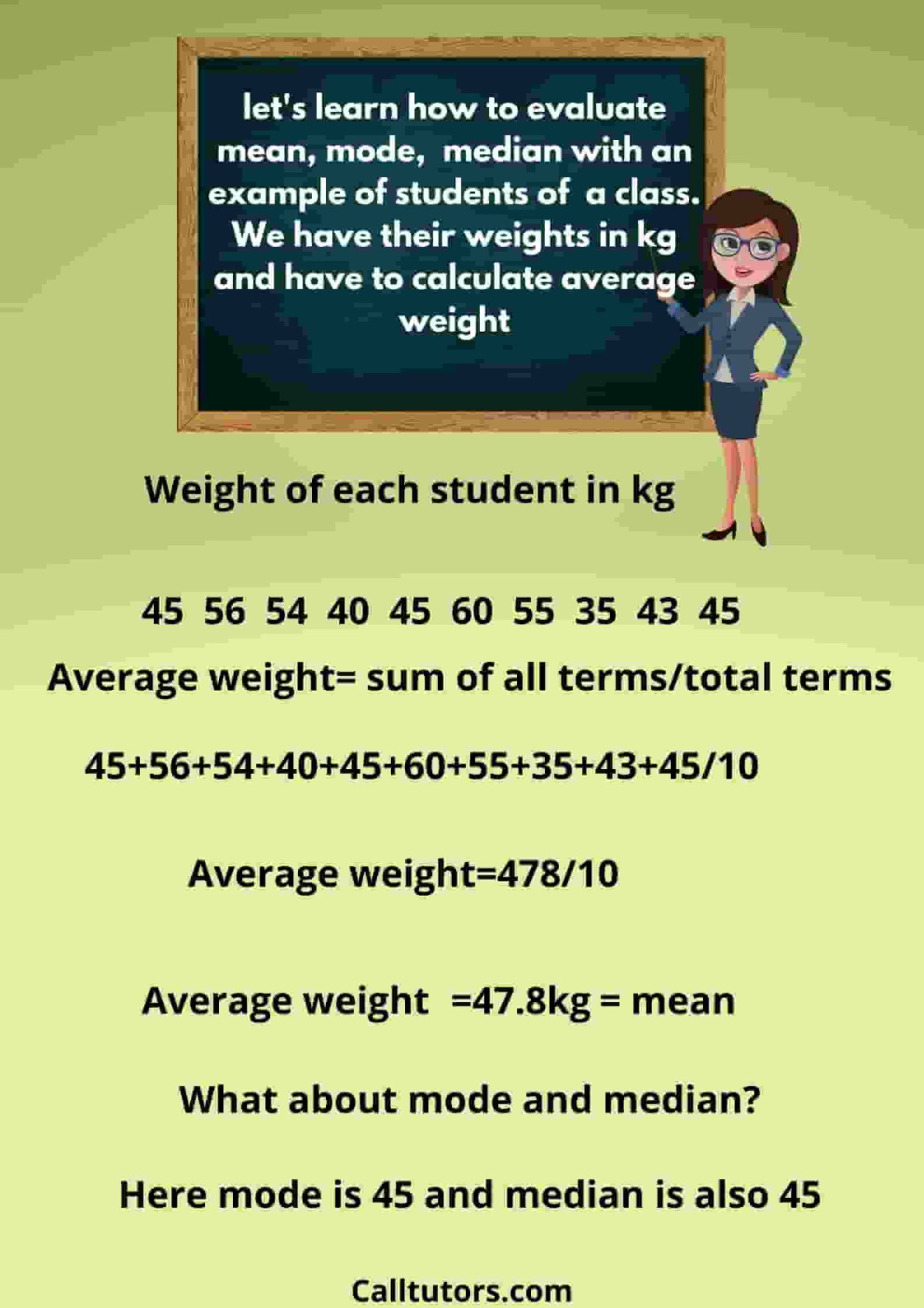
Average weight- We can calculate average weight with the mean formula
Mean = sum of all terms/ total terms
Hence the average weight of students is 47.8 kg
Mode = the frequent term in the list is known as the median.
In the above question 45 is mode because it is repeated three times.
Median= The central term is known as median. But in this question we have ten terms and we have two middle terms.
Now the mean of these two terms is median. But before that we have to arrange the values in any order.
35 40 43 45 45 45 54 55 56 60
Here 45+45/2= 90/2 = 45 is median
Hence to solve statistics problems you should know these formulas or tactics.
In this competitive world, data analysis is the key stream to earn more profits and to beat the competition. Statistics is used for the same as it is the type of science which deals with data analysis and much more. Many people struggle with How to solve statistics problems so this article is inclined to that only. In case, if you need any help with statistics assignment , then you can get the best help from our statistics assignment helper .
In this blog we have also differentiate between statistical and non statistical questions so that you can better understand what statistics problems require.
What are the types of Statistics?
Statistics is mainly of two types-
Descriptive- It just describe what the data shows
Inferential- It helps in generalization of data and draws valuable conclusions.
What are the components of a statistics problem?
- Ask a question
- Gather Data
- Data analysis
- Interpret Results
Which formulas should we know about how to solve statistics problems?
In statistics, we use numerous formulas to solve the different problems. Statistics problems require simple as well as complex formulas to give answers. We have to use formulas of mean, mode, median, and other probability formulas in statistics.
Similar Articles

13 Best Tips To Write An Assignment
Whenever the new semester starts, you will get a lot of assignment writing tasks. Now you enter the new academic…

How To Do Homework Fast – 11 Tips To Do Homework Fast
Homework is one of the most important parts that have to be done by students. It has been around for…
Leave a Comment Cancel Reply
Your email address will not be published. Required fields are marked *
This site uses Akismet to reduce spam. Learn how your comment data is processed .
ORIGINAL RESEARCH article
Statistical analysis of complex problem-solving process data: an event history analysis approach.

- 1 Department of Statistics, London School of Economics and Political Science, London, United Kingdom
- 2 School of Statistics, University of Minnesota, Minneapolis, MN, United States
- 3 Department of Statistics, Columbia University, New York, NY, United States
Complex problem-solving (CPS) ability has been recognized as a central 21st century skill. Individuals' processes of solving crucial complex problems may contain substantial information about their CPS ability. In this paper, we consider the prediction of duration and final outcome (i.e., success/failure) of solving a complex problem during task completion process, by making use of process data recorded in computer log files. Solving this problem may help answer questions like “how much information about an individual's CPS ability is contained in the process data?,” “what CPS patterns will yield a higher chance of success?,” and “what CPS patterns predict the remaining time for task completion?” We propose an event history analysis model for this prediction problem. The trained prediction model may provide us a better understanding of individuals' problem-solving patterns, which may eventually lead to a good design of automated interventions (e.g., providing hints) for the training of CPS ability. A real data example from the 2012 Programme for International Student Assessment (PISA) is provided for illustration.
1. Introduction
Complex problem-solving (CPS) ability has been recognized as a central 21st century skill of high importance for several outcomes including academic achievement ( Wüstenberg et al., 2012 ) and workplace performance ( Danner et al., 2011 ). It encompasses a set of higher-order thinking skills that require strategic planning, carrying out multi-step sequences of actions, reacting to a dynamically changing system, testing hypotheses, and, if necessary, adaptively coming up with new hypotheses. Thus, there is almost no doubt that an individual's problem-solving process data contain substantial amount of information about his/her CPS ability and thus are worth analyzing. Meaningful information extracted from CPS process data may lead to better understanding, measurement, and even training of individuals' CPS ability.
Problem-solving process data typically have a more complex structure than that of panel data which are traditionally more commonly encountered in statistics. Specifically, individuals may take different strategies toward solving the same problem. Even for individuals who take the same strategy, their actions and time-stamps of the actions may be very different. Due to such heterogeneity and complexity, classical regression and multivariate data analysis methods cannot be straightforwardly applied to CPS process data.
Possibly due to the lack of suitable analytic tools, research on CPS process data is limited. Among the existing works, none took a prediction perspective. Specifically, Greiff et al. (2015) presented a case study, showcasing the strong association between a specific strategic behavior (identified by expert knowledge) in a CPS task from the 2012 Programme for International Student Assessment (PISA) and performance both in this specific task and in the overall PISA problem-solving score. He and von Davier (2015 , 2016) proposed an N-gram method from natural language processing for analyzing problem-solving items in technology-rich environments, focusing on identifying feature sequences that are important to task completion. Vista et al. (2017) developed methods for the visualization and exploratory analysis of students' behavioral pathways, aiming to detect action sequences that are potentially relevant for establishing particular paths as meaningful markers of complex behaviors. Halpin and De Boeck (2013) and Halpin et al. (2017) adopted a Hawkes process approach to analyzing collaborative problem-solving items, focusing on the psychological measurement of collaboration. Xu et al. (2018) proposed a latent class model that analyzes CPS patterns by classifying individuals into latent classes based on their problem-solving processes.
In this paper, we propose to analyze CPS process data from a prediction perspective. As suggested in Yarkoni and Westfall (2017) , an increased focus on prediction can ultimately lead us to greater understanding of human behavior. Specifically, we consider the simultaneous prediction of the duration and the final outcome (i.e., success/failure) of solving a complex problem based on CPS process data. Instead of a single prediction, we hope to predict at any time during the problem-solving process. Such a data-driven prediction model may bring us insights about individuals' CPS behavioral patterns. First, features that contribute most to the prediction may correspond to important strategic behaviors that are key to succeeding in a task. In this sense, the proposed method can be used as an exploratory data analysis tool for extracting important features from process data. Second, the prediction accuracy may also serve as a measure of the strength of the signal contained in process data that reflects one's CPS ability, which reflects the reliability of CPS tasks from a prediction perspective. Third, for low stake assessments, the predicted chance of success may be used to give partial credits when scoring task takers. Fourth, speed is another important dimension of complex problem solving that is closely associated with the final outcome of task completion ( MacKay, 1982 ). The prediction of the duration throughout the problem-solving process may provide us insights on the relationship between the CPS behavioral patterns and the CPS speed. Finally, the prediction model also enables us to design suitable interventions during their problem-solving processes. For example, a hint may be provided when a student is predicted having a high chance to fail after sufficient efforts.
More precisely, we model the conditional distribution of duration time and final outcome given the event history up to any time point. This model can be viewed as a special event history analysis model, a general statistical framework for analyzing the expected duration of time until one or more events happen (see e.g., Allison, 2014 ). The proposed model can be regarded as an extension to the classical regression approach. The major difference is that the current model is specified over a continuous-time domain. It consists of a family of conditional models indexed by time, while the classical regression approach does not deal with continuous-time information. As a result, the proposed model supports prediction at any time during one's problem-solving process, while the classical regression approach does not. The proposed model is also related to, but substantially different from response time models (e.g., van der Linden, 2007 ) which have received much attention in psychometrics in recent years. Specifically, response time models model the joint distribution of response time and responses to test items, while the proposed model focuses on the conditional distribution of CPS duration and final outcome given the event history.
Although the proposed method learns regression-type models from data, it is worth emphasizing that we do not try to make statistical inference, such as testing whether a specific regression coefficient is significantly different from zero. Rather, the selection and interpretation of the model are mainly justified from a prediction perspective. This is because statistical inference tends to draw strong conclusions based on strong assumptions on the data generation mechanism. Due to the complexity of CPS process data, a statistical model may be severely misspecified, making valid statistical inference a big challenge. On the other hand, the prediction framework requires less assumptions and thus is more suitable for exploratory analysis. More precisely, the prediction framework admits the discrepancy between the underlying complex data generation mechanism and the prediction model ( Yarkoni and Westfall, 2017 ). A prediction model aims at achieving a balance between the bias due to this discrepancy and the variance due to a limited sample size. As a price, findings from the predictive framework are preliminary and only suggest hypotheses for future confirmatory studies.
The rest of the paper is organized as follows. In Section 2, we describe the structure of complex problem-solving process data and then motivate our research questions, using a CPS item from PISA 2012 as an example. In Section 3, we formulate the research questions under a statistical framework, propose a model, and then provide details of estimation and prediction. The introduced model is illustrated through an application to an example item from PISA 2012 in Section 4. We discuss limitations and future directions in Section 5.
2. Complex Problem-Solving Process Data
2.1. a motivating example.
We use a specific CPS item, CLIMATE CONTROL (CC) 1 , to demonstrate the data structure and to motivate our research questions. It is part of a CPS unit in PISA 2012 that was designed under the “MicroDYN” framework ( Greiff et al., 2012 ; Wüstenberg et al., 2012 ), a framework for the development of small dynamic systems of causal relationships for assessing CPS.
In this item, students are instructed to manipulate the panel (i.e., to move the top, central, and bottom control sliders; left side of Figure 1A ) and to answer how the input variables (control sliders) are related to the output variables (temperature and humidity). Specifically, the initial position of each control slider is indicated by a triangle “▴.” The students can change the top, central and bottom controls on the left of Figure 1 by using the sliders. By clicking “APPLY,” they will see the corresponding changes in temperature and humidity. After exploration, the students are asked to draw lines in a diagram ( Figure 1B ) to answer what each slider controls. The item is considered correctly answered if the diagram is correctly completed. The problem-solving process for this item is that the students must experiment to determine which controls have an impact on temperature and which on humidity, and then represent the causal relations by drawing arrows between the three inputs (top, central, and bottom control sliders) and the two outputs (temperature and humidity).

Figure 1. (A) Simulation environment of CC item. (B) Answer diagram of CC item.
PISA 2012 collected students' problem-solving process data in computer log files, in the form of a sequence of time-stamped events. We illustrate the structure of data in Table 1 and Figure 2 , where Table 1 tabulates a sequence of time-stamped events from a student and Figure 2 visualizes the corresponding event time points on a time line. According to the data, 14 events were recorded between time 0 (start) and 61.5 s (success). The first event happened at 29.5 s that was clicking “APPLY” after the top, central, and bottom controls were set at 2, 0, and 0, respectively. A sequence of actions followed the first event and finally at 58, 59.1, and 59.6 s, a final answer was correctly given using the diagram. It is worth clarifying that this log file does not collect all the interactions between a student and the simulated system. That is, the status of the control sliders is only recorded in the log file, when the “APPLY” button is clicked.

Table 1 . An example of computer log file data from CC item in PISA 2012.

Figure 2 . Visualization of the structure of process data from CC item in PISA 2012.
The process data for solving a CPS item typically have two components, knowledge acquisition and knowledge application, respectively. This CC item mainly focuses the former, which includes learning the causal relationships between the inputs and the outputs and representing such relationships by drawing the diagram. Since data on representing the causal relationship is relatively straightforward, in the rest of the paper, we focus on the process data related to knowledge acquisition and only refer a student's problem-solving process to his/her process of exploring the air conditioner, excluding the actions involving the answer diagram.
Intuitively, students' problem-solving processes contain information about their complex problem-solving ability, whether in the context of the CC item or in a more general sense of dealing with complex tasks in practice. However, it remains a challenge to extract meaningful information from their process data, due to the complex data structure. In particular, the occurrences of events are heterogeneous (i.e., different people can have very different event histories) and unstructured (i.e., there is little restriction on the order and time of the occurrences). Different students tend to have different problem-solving trajectories, with different actions taken at different time points. Consequently, time series models, which are standard statistical tools for analyzing dynamic systems, are not suitable here.
2.2. Research Questions
We focus on two specific research questions. Consider an individual solving a complex problem. Given that the individual has spent t units of time and has not yet completed the task, we would like to ask the following two questions based on the information at time t : How much additional time does the individual need? And will the individual succeed or fail upon the time of task completion?
Suppose we index the individual by i and let T i be the total time of task completion and Y i be the final outcome. Moreover, we denote H i ( t ) = ( h i 1 ( t ) , ... , h i p ( t ) ) ⊤ as a p -vector function of time t , summarizing the event history of individual i from the beginning of task to time t . Each component of H i ( t ) is a feature constructed from the event history up to time t . Taking the above CC item as an example, components of H i ( t ) may be, the number of actions a student has taken, whether all three control sliders have been explored, the frequency of using the reset button, etc., up to time t . We refer to H i ( t ) as the event history process of individual i . The dimension p may be high, depending on the complexity of the log file.
With the above notation, the two questions become to simultaneously predict T i and Y i based on H i ( t ). Throughout this paper, we focus on the analysis of data from a single CPS item. Extensions of the current framework to multiple-item analysis are discussed in Section 5.
3. Proposed Method
3.1. a regression model.
We now propose a regression model to answer the two questions raised in Section 2.2. We specify the marginal conditional models of Y i and T i given H i ( t ) and T i > t , respectively. Specifically, we assume
where Φ is the cumulative distribution function of a standard normal distribution. That is, Y i is assumed to marginally follow a probit regression model. In addition, only the conditional mean and variance are assumed for log( T i − t ). Our model parameters include the regression coefficients B = ( b jk )2 × p and conditional variance σ 2 . Based on the above model specification, a pseudo-likelihood function will be devived in Section 3.3 for parameter estimation.
Although only marginal models are specified, we point out that the model specifications (1) through (3) impose quite strong assumptions. As a result, the model may not most closely approximate the data-generating process and thus a bias is likely to exist. On the other hand, however, it is a working model that leads to reasonable prediction and can be used as a benchmark model for this prediction problem in future investigations.
We further remark that the conditional variance of log( T i − t ) is time-invariant under the current specification, which can be further relaxed to be time-dependent. In addition, the regression model for response time is closely related to the log-normal model for response time analysis in psychometrics (e.g., van der Linden, 2007 ). The major difference is that the proposed model is not a measurement model disentangling item and person effects on T i and Y i .
3.2. Prediction
Under the model in Section 3.1, given the event history, we predict the final outcome based on the success probability Φ( b 11 h i 1 ( t ) + ⋯ + b 1 p h ip ( t )). In addition, based on the conditional mean of log( T i − t ), we predict the total time at time t by t + exp( b 21 h i 1 ( t ) + ⋯ + b 2 p h ip ( t )). Given estimates of B from training data, we can predict the problem-solving duration and final outcome at any t for an individual in the testing sample, throughout his/her entire problem-solving process.
3.3. Parameter Estimation
It remains to estimate the model parameters based on a training dataset. Let our data be (τ i , y i ) and { H i ( t ): t ≥ 0}, i = 1, …, N , where τ i and y i are realizations of T i and Y i , and { H i ( t ): t ≥ 0} is the entire event history.
We develop estimating equations based on a pseudo likelihood function. Specifically, the conditional distribution of Y i given H i ( t ) and T i > t can be written as
where b 2 = ( b 11 , ... , b 1 p ) ⊤ . In addition, using the log-normal model as a working model for T i − t , the corresponding conditional distribution of T i can be written as
where b 2 = ( b 21 , ... , b 2 p ) ⊤ . The pseudo-likelihood is then written as
where t 1 , …, t J are J pre-specified grid points that spread out over the entire time spectrum. The choice of the grid points will be discussed in the sequel. By specifying the pseudo-likelihood based on the sequence of time points, the prediction at different time is taken into accounting in the estimation. We estimate the model parameters by maximizing the pseudo-likelihood function L ( B , σ).
In fact, (5) can be factorized into
Therefore, b 1 is estimated by maximizing L 1 ( b 1 ), which takes the form of a likelihood function for probit regression. Similarly, b 2 and σ are estimated by maximizing L 2 ( b 2 , σ), which is equivalent to solving the following estimation equations,
The estimating equations (8) and (9) can also be derived directly based on the conditional mean and variance specification of log( T i − t ). Solving these equations is equivalent to solving a linear regression problem, and thus is computationally easy.
3.4. Some Remarks
We provide a few remarks. First, choosing suitable features into H i ( t ) is important. The inclusion of suitable features not only improves the prediction accuracy, but also facilitates the exploratory analysis and interpretation of how behavioral patterns affect CPS result. If substantive knowledge about a CPS task is available from cognition theory, one may choose features that indicate different strategies toward solving the task. Otherwise, a data-driven approach may be taken. That is, one may select a model from a candidate list based on certain cross-validation criteria, where, if possible, all reasonable features should be consider as candidates. Even when a set of features has been suggested by cognition theory, one can still take the data-driven approach to find additional features, which may lead to new findings.
Second, one possible extension of the proposed model is to allow the regression coefficients to be a function of time t , whereas they are independent of time under the current model. In that case, the regression coefficients become functions of time, b jk ( t ). The current model can be regarded as a special case of this more general model. In particular, if b jk ( t ) has high variation along time in the best predictive model, then simply applying the current model may yield a high bias. Specifically, in the current estimation procedure, a larger grid point tends to have a smaller sample size and thus contributes less to the pseudo-likelihood function. As a result, a larger bias may occur in the prediction at a larger time point. However, the estimation of the time-dependent coefficient is non-trivial. In particular, constraints should be imposed on the functional form of b jk ( t ) to ensure a certain level of smoothness over time. As a result, b jk ( t ) can be accurately estimated using information from a finite number of time points. Otherwise, without any smoothness assumptions, to predict at any time during one's problem-solving process, there are an infinite number of parameters to estimate. Moreover, when a regression coefficient is time-dependent, its interpretation becomes more difficult, especially if the sign changes over time.
Third, we remark on the selection of grid points in the estimation procedure. Our model is specified in a continuous time domain that supports prediction at any time point in a continuum during an individual's problem-solving process. The use of discretized grid points is a way to approximate the continuous-time system, so that estimation equations can be written down. In practice, we suggest to place the grid points based on the quantiles of the empirical distribution of duration based on the training set. See the analysis in Section 4 for an illustration. The number of grid points may be further selected by cross validation. We also point out that prediction can be made at any time point on the continuum, not limited to the grid points for parameter estimation.
4. An Example from PISA 2012
4.1. background.
In what follows, we illustrate the proposed method via an application to the above CC item 2 . This item was also analyzed in Greiff et al. (2015) and Xu et al. (2018) . The dataset was cleaned from the entire released dataset of PISA 2012. It contains 16,872 15-year-old students' problem-solving processes, where the students were from 42 countries and economies. Among these students, 54.5% answered correctly. On average, each student took 129.9 s and 17 actions solving the problem. Histograms of the students' problem-solving duration and number of actions are presented in Figure 3 .

Figure 3. (A) Histogram of problem-solving duration of the CC item. (B) Histogram of the number of actions for solving the CC item.
4.2. Analyses
The entire dataset was randomly split into training and testing sets, where the training set contains data from 13,498 students and the testing set contains data from 3,374 students. A predictive model was built solely based on the training set and then its performance was evaluated based on the testing set. We used J = 9 grid points for the parameter estimation, with t 1 through t 9 specified to be 64, 81, 94, 106, 118, 132, 149, 170, and 208 s, respectively, which are the 10% through 90% quantiles of the empirical distribution of duration. As discussed earlier, the number of grid points and their locations may be further engineered by cross validation.
4.2.1. Model Selection
We first build a model based on the training data, using a data-driven stepwise forward selection procedure. In each step, we add one feature into H i ( t ) that leads to maximum increase in a cross-validated log-pseudo-likelihood, which is calculated based on a five-fold cross validation. We stop adding features into H i ( t ) when the cross-validated log-pseudo-likelihood stops increasing. The order in which the features are added may serve as a measure of their contribution to predicting the CPS duration and final outcome.
The candidate features being considered for model selection are listed in Table 2 . These candidate features were chosen to reflect students' CPS behavioral patterns from different aspects. In what follows, we discuss some of them. For example, the feature I i ( t ) indicates whether or not all three control sliders have been explored by simple actions (i.e., moving one control slider at a time) up to time t . That is, I i ( t ) = 1 means that the vary-one-thing-at-a-time (VOTAT) strategy ( Greiff et al., 2015 ) has been taken. According to the design of the CC item, the VOTAT strategy is expected to be a strong predictor of task success. In addition, the feature N i ( t )/ t records a student's average number of actions per unit time. It may serve as a measure of the student's speed of taking actions. In experimental psychology, response time or equivalently speed has been a central source for inferences about the organization and structure of cognitive processes (e.g., Luce, 1986 ), and in educational psychology, joint analysis of speed and accuracy of item response has also received much attention in recent years (e.g., van der Linden, 2007 ; Klein Entink et al., 2009 ). However, little is known about the role of speed in CPS tasks. The current analysis may provide some initial result on the relation between a student's speed and his/her CPS performance. Moreover, the features defined by the repeating of previously taken actions may reflect students' need of verifying the derived hypothesis on the relation based on the previous action or may be related to students' attention if the same actions are repeated many times. We also include 1, t, t 2 , and t 3 in H i ( t ) as the initial set of features to capture the time effect. For simplicity, country information is not taken into account in the current analysis.

Table 2 . The list of candidate features to be incorporated into the model.
Our results on model selection are summarized in Figure 4 and Table 3 . The pseudo-likelihood stopped increasing after 11 steps, resulting a final model with 15 components in H i ( t ). As we can see from Figure 4 , the increase in the cross-validated log-pseudo-likelihood is mainly contributed by the inclusion of features in the first six steps, after which the increment is quite marginal. As we can see, the first, second, and sixth features entering into the model are all related to taking simple actions, a strategy known to be important to this task (e.g., Greiff et al., 2015 ). In particular, the first feature being selected is I i ( t ), which confirms the strong effect of the VOTAT strategy. In addition, the third and fourth features are both based on N i ( t ), the number of actions taken before time t . Roughly, the feature 1 { N i ( t )>0} reflects the initial planning behavior ( Eichmann et al., 2019 ). Thus, this feature tends to measure students' speed of reading the instruction of the item. As discussed earlier, the feature N i ( t )/ t measures students' speed of taking actions. Finally, the fifth feature is related to the use of the RESET button.

Figure 4 . The increase in the cross-validated log-pseudo-likelihood based on a stepwise forward selection procedure. (A–C) plot the cross-validated log-pseudo-likelihood, corresponding to L ( B , σ), L 1 ( b 1 ), L 2 ( b 2 , σ), respectively.

Table 3 . Results on model selection based on a stepwise forward selection procedure.
4.2.2. Prediction Performance on Testing Set
We now look at the prediction performance of the above model on the testing set. The prediction performance was evaluated at a larger set of time points from 19 to 281 s. Instead of reporting based on the pseudo-likelihood function, we adopted two measures that are more straightforward. Specifically, we measured the prediction of final outcome by the Area Under the Curve (AUC) of the predicted Receiver Operating Characteristic (ROC) curve. The value of AUC is between 0 and 1. A larger AUC value indicates better prediction of the binary final outcome, with AUC = 1 indicating perfect prediction. In addition, at each time point t , we measured the prediction of duration based on the root mean squared error (RMSE), defined as
where τ i , i = N + 1, …, N + n , denotes the duration of students in the testing set, and τ ^ i ( t ) denotes the prediction based on information up to time t according to the trained model.
Results are presented in Figure 5 , where the testing AUC and RMSE for the final outcome and duration are presented. In particular, results based on the model selected by cross validation ( p = 15) and the initial model ( p = 4, containing the initial covariates 1, t , t 2 , and t 3 ) are compared. First, based on the selected model, the AUC is never above 0.8 and the RMSE is between 53 and 64 s, indicating a low signal-to-noise ratio. Second, the students' event history does improve the prediction of final outcome and duration upon the initial model. Specifically, since the initial model does not take into account the event history, it predicts the students with duration longer than t to have the same success probability. Consequently, the test AUC is 0.5 at each value of t , which is always worse than the performance of the selected model. Moreover, the selected model always outperforms the initial model in terms of the prediction of duration. Third, the AUC for the prediction of the final outcome is low when t is small. It keeps increasing as time goes on and fluctuates around 0.72 after about 120 s.

Figure 5 . A comparison of prediction accuracy between the model selected by cross validation and a baseline model without using individual specific event history.
4.2.3. Interpretation of Parameter Estimates
To gain more insights into how the event history affects the final outcome and duration, we further look at the results of parameter estimation. We focus on a model whose event history H i ( t ) includes the initial features and the top six features selected by cross validation. This model has similar prediction accuracy as the selected model according to the cross-validation result in Figure 4 , but contains less features in the event history and thus is easier to interpret. Moreover, the parameter estimates under this model are close to those under the cross-validation selected model, and the signs of the regression coefficients remain the same.
The estimated regression coefficients are presented in Table 4 . First, the first selected feature I i ( t ), which indicates whether all three control sliders have been explored via simple actions, has a positive regression coefficient on final outcome and a negative coefficient on duration. It means that, controlling the rest of the parameters, a student who has taken the VOTAT strategy tends to be more likely to give a correct answer and to complete in a shorter period of time. This confirms the strong effect of VOTAT strategy in solving the current task.

Table 4 . Estimated regression coefficients for a model for which the event history process contains the initial features based on polynomials of t and the top six features selected by cross validation.
Second, besides I i ( t ), there are two features related to taking simple actions, 1 { S i ( t )>0} and S i ( t )/ t , which are the indicator of taking at least one simple action and the frequency of taking simple actions. Both features have positive regression coefficients on the final outcome, implying larger values of both features lead to a higher success rate. In addition, 1 { S i ( t )>0} has a negative coefficient on duration and S i ( t )/ t has a positive one. Under this estimated model, the overall simple action effect on duration is b ^ 25 I i ( t ) + b ^ 26 1 { S i ( t ) > 0 } + b ^ 2 , 10 S i ( t ) / t , which is negative for most students. It implies that, overall, taking simple actions leads to a shorter predicted duration. However, once all three types of simple actions have been taken, a higher frequency of taking simple actions leads to a weaker but sill negative simple action effect on the duration.
Third, as discussed earlier, 1 { N i ( t )>0} tends to measure the student's speed of reading the instruction of the task and N i ( t )/ t can be regarded as a measure of students' speed of taking actions. According to the estimated regression coefficients, the data suggest that a student who reads and acts faster tends to complete the task in a shorter period of time with a lower accuracy. Similar results have been seen in the literature of response time analysis in educational psychology (e.g., Klein Entink et al., 2009 ; Fox and Marianti, 2016 ; Zhan et al., 2018 ), where speed of item response was found to negatively correlated with accuracy. In particular, Zhan et al. (2018) found a moderate negative correlation between students' general mathematics ability and speed under a psychometric model for PISA 2012 computer-based mathematics data.
Finally, 1 { R i ( t )>0} , the use of the RESET button, has positive regression coefficients on both final outcome and duration. It implies that the use of RESET button leads to a higher predicted success probability and a longer duration time, given the other features controlled. The connection between the use of the RESET button and the underlying cognitive process of complex problem solving, if it exists, still remains to be investigated.
5. Discussions
5.1. summary.
As an early step toward understanding individuals' complex problem-solving processes, we proposed an event history analysis method for the prediction of the duration and the final outcome of solving a complex problem based on process data. This approach is able to predict at any time t during an individual's problem-solving process, which may be useful in dynamic assessment/learning systems (e.g., in a game-based assessment system). An illustrative example is provided that is based on a CPS item from PISA 2012.
5.2. Inference, Prediction, and Interpretability
As articulated previously, this paper focuses on a prediction problem, rather than a statistical inference problem. Comparing with a prediction framework, statistical inference tends to draw stronger conclusions under stronger assumptions on the data generation mechanism. Unfortunately, due to the complexity of CPS process data, such assumptions are not only hardly satisfied, but also difficult to verify. On the other hand, a prediction framework requires less assumptions and thus is more suitable for exploratory analysis. As a price, the findings from the predictive framework are preliminary and can only be used to generate hypotheses for future studies.
It may be useful to provide uncertainty measures for the prediction performance and for the parameter estimates, where the former indicates the replicability of the prediction performance and the later reflects the stability of the prediction model. In particular, patterns from a prediction model with low replicability and low stability should not be overly interpreted. Such uncertainty measures may be obtained from cross validation and bootstrapping (see Chapter 7, Friedman et al., 2001 ).
It is also worth distinguishing prediction methods based on a simple model like the one proposed above and those based on black-box machine learning algorithms (e.g., random forest). Decisions based on black-box algorithms can be very difficult to understood by human and thus do not provide us insights about the data, even though they may have a high prediction accuracy. On the other hand, a simple model can be regarded as a data dimension reduction tool that extracts interpretable information from data, which may facilitate our understanding of complex problem solving.
5.3. Extending the Current Model
The proposed model can be extended along multiple directions. First, as discussed earlier, we may extend the model by allowing the regression coefficients b jk to be time-dependent. In that case, nonparametric estimation methods (e.g., splines) need to be developed for parameter estimation. In fact, the idea of time-varying coefficients has been intensively investigated in the event history analysis literature (e.g., Fan et al., 1997 ). This extension will be useful if the effects of the features in H i ( t ) change substantially over time.
Second, when the dimension p of H i ( t ) is high, better interpretability and higher prediction power may be achieved by using Lasso-type sparse estimators (see e.g., Chapter 3 Friedman et al., 2001 ). These estimators perform simultaneous feature selection and regularization in order to enhance the prediction accuracy and interpretability.
Finally, outliers are likely to occur in the data due to the abnormal behavioral patterns of a small proportion of people. A better treatment of outliers will lead to better prediction performance. Thus, a more robust objective function will be developed for parameter estimation, by borrowing ideas from the literature of robust statistics (see e.g., Huber and Ronchetti, 2009 ).
5.4. Multiple-Task Analysis
The current analysis focuses on analyzing data from a single task. To study individuals' CPS ability, it may be of more interest to analyze multiple CPS tasks simultaneously and to investigate how an individual's process data from one or multiple tasks predict his/her performance on the other tasks. Generally speaking, one's CPS ability may be better measured by the information in the process data that is generalizable across a representative set of CPS tasks than only his/her final outcomes on these tasks. In this sense, this cross-task prediction problem is closely related to the measurement of CPS ability. This problem is also worth future investigation.
Author Contributions
All authors listed have made a substantial, direct and intellectual contribution to the work, and approved it for publication.
This research was funded by NAEd/Spencer postdoctoral fellowship, NSF grant DMS-1712657, NSF grant SES-1826540, NSF grant IIS-1633360, and NIH grant R01GM047845.
Conflict of Interest Statement
The authors declare that the research was conducted in the absence of any commercial or financial relationships that could be construed as a potential conflict of interest.
1. ^ The item can be found on the OECD website ( http://www.oecd.org/pisa/test-2012/testquestions/question3/ )
2. ^ The log file data and code book for the CC item can be found online: http://www.oecd.org/pisa/pisaproducts/database-cbapisa2012.htm .
Allison, P. D. (2014). Event history analysis: Regression for longitudinal event data . London: Sage.
Google Scholar
Danner, D., Hagemann, D., Schankin, A., Hager, M., and Funke, J. (2011). Beyond IQ: a latent state-trait analysis of general intelligence, dynamic decision making, and implicit learning. Intelligence 39, 323–334. doi: 10.1016/j.intell.2011.06.004
CrossRef Full Text | Google Scholar
Eichmann, B., Goldhammer, F., Greiff, S., Pucite, L., and Naumann, J. (2019). The role of planning in complex problem solving. Comput. Educ . 128, 1–12. doi: 10.1016/j.compedu.2018.08.004
Fan, J., Gijbels, I., and King, M. (1997). Local likelihood and local partial likelihood in hazard regression. Anna. Statist . 25, 1661–1690. doi: 10.1214/aos/1031594736
Fox, J.-P., and Marianti, S. (2016). Joint modeling of ability and differential speed using responses and response times. Multivar. Behav. Res . 51, 540–553. doi: 10.1080/00273171.2016.1171128
PubMed Abstract | CrossRef Full Text | Google Scholar
Friedman, J., Hastie, T., and Tibshirani, R. (2001). The Elements of Statistical Learning . New York, NY: Springer.
Greiff, S., Wüstenberg, S., and Avvisati, F. (2015). Computer-generated log-file analyses as a window into students' minds? A showcase study based on the PISA 2012 assessment of problem solving. Comput. Educ . 91, 92–105. doi: 10.1016/j.compedu.2015.10.018
Greiff, S., Wüstenberg, S., and Funke, J. (2012). Dynamic problem solving: a new assessment perspective. Appl. Psychol. Measur . 36, 189–213. doi: 10.1177/0146621612439620
Halpin, P. F., and De Boeck, P. (2013). Modelling dyadic interaction with Hawkes processes. Psychometrika 78, 793–814. doi: 10.1007/s11336-013-9329-1
Halpin, P. F., von Davier, A. A., Hao, J., and Liu, L. (2017). Measuring student engagement during collaboration. J. Educ. Measur . 54, 70–84. doi: 10.1111/jedm.12133
He, Q., and von Davier, M. (2015). “Identifying feature sequences from process data in problem-solving items with N-grams,” in Quantitative Psychology Research , eds L. van der Ark, D. Bolt, W. Wang, J. Douglas, and M. Wiberg, (New York, NY: Springer), 173–190.
He, Q., and von Davier, M. (2016). “Analyzing process data from problem-solving items with n-grams: insights from a computer-based large-scale assessment,” in Handbook of Research on Technology Tools for Real-World Skill Development , eds Y. Rosen, S. Ferrara, and M. Mosharraf (Hershey, PA: IGI Global), 750–777.
Huber, P. J., and Ronchetti, E. (2009). Robust Statistics . Hoboken, NJ: John Wiley & Sons.
Klein Entink, R. H., Kuhn, J.-T., Hornke, L. F., and Fox, J.-P. (2009). Evaluating cognitive theory: A joint modeling approach using responses and response times. Psychol. Methods 14, 54–75. doi: 10.1037/a0014877
Luce, R. D. (1986). Response Times: Their Role in Inferring Elementary Mental Organization . New York, NY: Oxford University Press.
MacKay, D. G. (1982). The problems of flexibility, fluency, and speed–accuracy trade-off in skilled behavior. Psychol. Rev . 89, 483–506. doi: 10.1037/0033-295X.89.5.483
van der Linden, W. J. (2007). A hierarchical framework for modeling speed and accuracy on test items. Psychometrika 72, 287–308. doi: 10.1007/s11336-006-1478-z
Vista, A., Care, E., and Awwal, N. (2017). Visualising and examining sequential actions as behavioural paths that can be interpreted as markers of complex behaviours. Comput. Hum. Behav . 76, 656–671. doi: 10.1016/j.chb.2017.01.027
Wüstenberg, S., Greiff, S., and Funke, J. (2012). Complex problem solving–More than reasoning? Intelligence 40, 1–14. doi: 10.1016/j.intell.2011.11.003
Xu, H., Fang, G., Chen, Y., Liu, J., and Ying, Z. (2018). Latent class analysis of recurrent events in problem-solving items. Appl. Psychol. Measur . 42, 478–498. doi: 10.1177/0146621617748325
Yarkoni, T., and Westfall, J. (2017). Choosing prediction over explanation in psychology: lessons from machine learning. Perspect. Psychol. Sci . 12, 1100–1122. doi: 10.1177/1745691617693393
Zhan, P., Jiao, H., and Liao, D. (2018). Cognitive diagnosis modelling incorporating item response times. Br. J. Math. Statist. Psychol . 71, 262–286. doi: 10.1111/bmsp.12114
Keywords: process data, complex problem solving, PISA data, response time, event history analysis
Citation: Chen Y, Li X, Liu J and Ying Z (2019) Statistical Analysis of Complex Problem-Solving Process Data: An Event History Analysis Approach. Front. Psychol . 10:486. doi: 10.3389/fpsyg.2019.00486
Received: 31 August 2018; Accepted: 19 February 2019; Published: 18 March 2019.
Reviewed by:
Copyright © 2019 Chen, Li, Liu and Ying. This is an open-access article distributed under the terms of the Creative Commons Attribution License (CC BY) . The use, distribution or reproduction in other forums is permitted, provided the original author(s) and the copyright owner(s) are credited and that the original publication in this journal is cited, in accordance with accepted academic practice. No use, distribution or reproduction is permitted which does not comply with these terms.
*Correspondence: Yunxiao Chen, [email protected]
Disclaimer: All claims expressed in this article are solely those of the authors and do not necessarily represent those of their affiliated organizations, or those of the publisher, the editors and the reviewers. Any product that may be evaluated in this article or claim that may be made by its manufacturer is not guaranteed or endorsed by the publisher.

Query Exercise: Solving The 201 Buckets Problem
When you run a query, SQL Server needs to estimate the number of matching rows it’ll find – so that it can decide which indexes to use, whether to go parallel, how much memory to grant, and more.
For example, take any Stack Overflow database , and let’s say I have an index on Location, and I want to find the top-ranking users in Lithuania:
| INDEX Location ON dbo.Users(Location); * FROM dbo.Users Location = N'lithuania' BY Reputation DESC; |
Then SQL Server has to guess how many people are in Lithuania so it can decide whether to use the index on Location, or do a table scan – because if there are a lot of folks in Lithuania, then it would mean a lot of key lookups to get the Reputation value for each of them.
We’ll run the query in the small StackOverflow2010 database and review the actual execution plan :

In the top right operator, the Index Seek, SQL Server only estimated 5 rows, but 84 rows actually came back. Now, that’s not really a problem for this particular query because:
- SQL Server used the index – which makes the query fast
- SQL Server did 84 key lookups instead of 5 – but still, that’s less logical reads than a table scan
- The query went single-threaded – but there was so little work that it didn’t matter
- The query didn’t spill to disk – there’s no yellow bang on the sort operator
As our database grows, though, the lines start to blur. Let’s run the same query on the largest current version of the StackOverflow database and see what happens in the actual execution plan :

The top right operator, the Index Seek, shows just 8 rows estimated, but 2,554 rows were actually found. As our data size grows, these estimate variances start to become problematic. Now granted, this succeeds in the same way the 2010 query succeeds: we get an index seek, it’s still less logical reads than a key lookup plan would be, the single-threaded thing isn’t a problem for a 27 millisecond query, and we don’t spill to disk.
However, if we start to join to other tables (and we will, in the next Query Exercise), then this under-estimation is going to become a problem.
Why is the estimate wrong?
We do indeed have statistics on the Location index, and they were created with fullscan since we just created the index. Let’s view the statistics for the large database:
| SHOW_STATISTICS('dbo.Users', 'Location') |
And check out the histogram contents – we’ll page down to Lithuania:

Or rather, we’ll page down to where you would expect Lithuania to be, and there’s a problem: Lithuania’s not there. SQL Server’s statistics are limited to just 201 buckets, max. (Technically, it’s up to 200 buckets for “normal” values in the table, plus 1 bucket for null.)
SQL Server does the best job it can of picking outliers in order to paint a perfect picture of the data, but it’s hard with just 201 buckets.
Typically – but not always – when SQL Server picks the locations that it’ll use for outliers, it uses around the top 200 locations by size, but this can vary a lot depending on the sort order of the column and the distribution of the data. Let’s look at the top locations:
| TOP 250 Location, COUNT(*) AS recs FROM dbo.Users GROUP BY Location ORDER BY COUNT(*) DESC; |
And Lithuania is at row 240 in this case:

So it’s a big location – but not big enough to hit the top 201 , which means it’s not going to get accurate estimates. The estimates are derived by looking at which bucket Lithuania is in – in the screenshot below, it’s row 100:
Lithuania is higher than Lisbon, but less than London, so it’s in the row 100 bucket. The row 100’s AVG_RANGE_ROWS is 7.847202, which means that any location between Lisbon and London has an average number of rows of about 8. And that’s where the estimate is coming from in our query:

Your challenge: get an accurate estimate.
You can change the query, the database, server-level settings, you name it. Anything that you would do in a real-life situation, you can do here. However, having done this exercise in my Mastering classes, I can tell you a couple things that people will try to do, but don’t really make sense.
You don’t wanna dump the data into a temp table first. Sometimes people will extract all of the data into a temp table, and then select data out of the temp table and say, “See, the estimate is accurate!” Sure it is, speedy, but look at your estimate from when you’re pulling the data out of the real table – the estimate’s still wrong there.
You don’t wanna use a hard-coded stat or index for just ‘Lithuania’. That only solves this one value, but you’ll still have the problem for every other outlier. We’re looking for a solution that we can use for most big outliers. (It’s always tricky to phrase question requirements in a way that rules out bad answers without pointing you to a specifically good answer, hahaha.)
Put your queries in a Github Gist and the query plans in PasteThePlan , showing your new accurate estimates , and include those link in your comments. Check out the solutions from other folks, and compare and contrast your work. I’ll circle back next week for a discussion on the answers. Have fun!
10 Comments . Leave new

My Gist https://gist.github.com/Paul-Fenton/83b0829263e9586868e1bd29fc2d6ccf
Query Plan https://www.brentozar.com/pastetheplan/?id=r19_spQjC
Create a new column “PopularLocation” which is set to the Location if it’s one of the top 250 locations.
Then change the query to look like:
SELECT * FROM dbo.Users WHERE Location = N’Lithuania’ OR PopularLocation = N’Lithuania’ ORDER BY Reputation DESC;
The estimate is now “84 of 85 rows (98%)” instead of “84 of 5 rows (1680%)”

I love the creativity! But…
Now the query is doing a table scan for just 84 rows. Check the estimates on other values, like India or San Diego

Sorry, cannot test it right now, just thinking out loud, perhaps filtered stats may solve it… I know it won’t probably work for other locations, but perhaps if we use parameter for the location, and using RECOMPILE hint that will be more accurate… Again sorry , but cannot test it right now…..
Uri, please reread the post more carefully and respect the time of others. Thank you.

Sometimes I need to cheat mssql because I want to see what will happen when there are many rows.
UPDATE STATISTICS dbo.Users([Location]) WITH rowcount =500000000000;
This gives 77 rows in Lithuanian. I known its not real life but for testing it is sometimes useful.
HAHAHA! That’s a funny idea, love it.

Code: https://gist.github.com/samot1/8d6e3bc5feee76b7959841cae8f81b97 Plan: https://www.brentozar.com/pastetheplan/?id=HJnkAt4oR
Idea: I just created a filtered statistic for every location starting with A, with B, with C … with Z
This way I have not just 200 statistic steps but 5200 which is enough to cover the most larger locations and get the correct estimates.
Drawback: you may or may not have to use OPTION(RECOMPILE) to use the correct statistic. When you put the location into a variable and use it in the query or have the PARAMETERIZATION option on your database set to FORCED you always have to use RECOMPILE to get the correct estimate.
PS: in a real scenario there may be much better options to archive the correct estimate, but you would need to know, how exactly the database is queried (which queries, how often, what happens with the results, how busy is the server …) and use all this information to decide the best option (which could be to simply ignore the wrong estimates too, since the overhead is bigger than the result)
Thomas – that is intriguing! I love the creativity.
I like the drawbacks that you put in the Gist – there are totally drawbacks here, for sure. For example, each stat has to be updated separately, so we just made our maintenance window explode. However, if someone is advanced enough to use this solution, I’d also expect them to be advanced enough to have relatively infrequent, targeted statistics updates.
I like it! I think you’ll also like the solution I talk about in next week’s post.
I had another much worse idea but it didn’t work (even if it could/should): CREATE PARTITION FUNCTION pf_a_to_z (NVARCHAR(100)) AS RANGE RIGHT FOR VALUES (‘A’, ‘B’, ‘C’, ‘D’, ‘E’, ‘F’, ‘G’, ‘H’, ‘I’, ‘J’, ‘K’, ‘L’, ‘M’, ‘N’, ‘O’, ‘P’, ‘Q’, ‘R’, ‘S’, ‘T’, ‘U’, ‘V’, ‘W’, ‘X’, ‘Y’, ‘Z’) CREATE PARTITION SCHEME ps_a_to_z AS PARTITION pf_a_to_z ALL TO ([PRIMARY]) ALTER TABLE [dbo].[Users] DROP CONSTRAINT [PK_Users_Id]; — drop old PK
CREATE UNIQUE CLUSTERED INDEX pk_Users_id ON dbo.Users (Id, Location) ON ps_a_to_z (Location) — base table (=clustered index) must be partition aligned, to allow STATISTICS_INCREMENTAL = ON on the location index GO CREATE NONCLUSTERED INDEX [Location] ON [dbo].[Users] ([Location]) WITH (DROP_EXISTING = ON, DATA_COMPRESSION = NONE, SORT_IN_TEMPDB = ON, ALLOW_ROW_LOCKS = ON, ALLOW_PAGE_LOCKS = ON, STATISTICS_INCREMENTAL = ON ) ON ps_a_to_z (Location); GO
now I have a table who is partitioned by the location, the STATISTICS_INCREMENTAL = ON says, that it should get one statistic per partition (plus a combined one), but sadly the SQL server eliminates the statistics all besides one but didn’t use the partitions statistic, so the estimates are still wrong.
And I have several drawbacks, e.g. I need to specifiy the location to be able to query the UserID efficent and I can have the same UserId twice in several locations, except I create another unique nonclustered index on the UserId …
[…] Query Exercise: Solving The 201 Buckets Problem (Brent Ozar) […]
And because you just have to get your two cents in: Cancel reply

Hi! I’m Brent Ozar.
I make Microsoft SQL Server go faster. I love teaching, travel, cars, and laughing. I’m based out of Las Vegas. He/him. I teach SQL Server training classes , or if you haven’t got time for the pain, I’m available for consulting too.
- Subscribe *
Insert/edit link
Enter the destination URL
Or link to existing content
IMAGES
COMMENTS
Statistics As Problem Solving. Consider statistics as a problem-solving process and examine its four components: asking questions, collecting appropriate data, analyzing the data, and interpreting the results. This session investigates the nature of data and its potential sources of variation. Variables, bias, and random sampling are introduced.
Part A: A Problem-Solving Process (15 minutes) The word statistics may bring to mind polls and surveys, or facts and figures in a newspaper article. But statistics is more than just a bunch of numbers: Statistics is a problem-solving process that seeks answers to questions through data. By asking and answering statistical questions, we can ...
For further ideas on statistical problem-solving, refer to a full guide on Common Statistical Errors. Tools for Solving Statistical Problems. When it comes to tackling statistical tough difficulties effectively, having the right tools at our disposal is important. Here are some key tools that can aid us in solving statistical problems:
Statistical Problem Solving. Problem solving in any organization is a problem. Nobody wants to own the responsibility for a problem and that is the reason, when a problem shows up fingers may be pointing at others rather than self. This is a natural human instinctive defense mechanism and hence cannot hold it against any one.
Problem 1. In one state, 52% of the voters are Republicans, and 48% are Democrats. In a second state, 47% of the voters are Republicans, and 53% are Democrats. Suppose a simple random sample of 100 voters are surveyed from each state. What is the probability that the survey will show a greater percentage of Republican voters in the second state ...
Statistical thinking is vital for solving real-world problems. At the heart of statistical thinking is making decisions based on data. This requires disciplined approaches to identifying problems and the ability to quantify and interpret the variation that you observe in your data. In this module, you will learn how to clearly define your ...
Statistical analysis means investigating trends, patterns, and relationships using quantitative data. It is an important research tool used by scientists, governments, businesses, and other organizations. To draw valid conclusions, statistical analysis requires careful planning from the very start of the research process. You need to specify ...
Welcome! Here, you will find all the help you need to be successful in your statistics class. Check out our statistics calculators to get step-by-step solutions to almost any statistics problem. Choose from topics such as numerical summary, confidence interval, hypothesis testing, simple regression and more.
There are 10 modules in this course. Statistical Thinking for Industrial Problem Solving is an applied statistics course for scientists and engineers offered by JMP, a division of SAS. By completing this course, students will understand the importance of statistical thinking, and will be able to use data and basic statistical methods to solve ...
Consider statistics as a problem-solving process and examine its four components: asking questions, collecting appropriate data, analyzing the data, and interpreting the results. This session investigates the nature of data and its potential sources of variation. Variables, bias, and random sampling are introduced.
Although there is much that is distinct about statistical problem solving, there is also much that is in common with mathematical problem solving so that statistics education researchers can learn a lot from work in mathematics education research and classic works such as Schoenfeld . When most statisticians hear "theory," they think ...
1. Plan (Ask a question): formulate a statistical question that can be answered with data. A good deal of time should be given to this step as it is the most important step in the process. 2. Collect (Produce Data): design and implement a plan to collect appropriate data. Data can be collected through numerous methods, such as observations, interviews, questionnaires, databases, samplings or ...
Statistical analysis is the process of collecting and analyzing large volumes of data in order to identify trends and develop valuable insights. In the professional world, statistical analysts take raw data and find correlations between variables to reveal patterns and trends to relevant stakeholders. Working in a wide range of different fields ...
The Shainin System™ (SS) is defined as a problem-solving system designed for medium- to high-volume processes where data are cheaply available, statistical methods are widely used, and intervention into the process is difficult. It has been mostly applied in parts and assembly operations facilities.
T/F Statistics is only used in the SOLVE step of statistical problem solving. False: Statistics is used in all four steps of statistical problem solving. T/F It is not necessary to compute values for statistical inference in the SOLVE step when inference is not being done.
The Six Sigma approach is a truly powerful problem-solving tool. By working from a practical problem to a statistical problem, a statistical solution and finally a practical solution, you will be assured that you have identified the correct root cause of the problem which affects the quality of your products.
Here is an example that helps you to understand the statistics problem easily. Almost 17 boys were diagnosed with a specific disease that leads to weight change. Here the data after family therapy was as follows: 11,11, 6, 9, 14, -3, 0, 7, 22, -5 , -4, 13, 13, 9, 4 , 6, 11 #2: Analyze the statistics problem. Once you assign the statistics ...
Free math problem solver answers your statistics homework questions with step-by-step explanations. Mathway. Visit Mathway on the web. Start 7-day free trial on the app. Start 7-day free trial on the app. Download free on Amazon. Download free in Windows Store. Take a photo of your math problem on the app. get Go. Statistics. Basic Math.
The 8D problem solving model establishes a permanent corrective action based on statistical analysis of the problem and focuses on the origin of the problem by determining its root causes. Although it originally comprised eight stages, or disciplines, the eight disciplines system was later augmented by an initial planning stage.
The general method of solving statistics problems is to write your question then collect data required for solving such a question and lastly you are required to analyse such data and to draw conclusion. Statistical and non-statistical problem. Let's know the difference between a statistical problem and non statistical problem.
Session 1 Statistics As Problem Solving. Consider statistics as a problem-solving process and examine its four components: asking questions, collecting appropriate data, analyzing the data, and interpreting the results. This session investigates the nature of data and its potential sources of variation. Variables, bias, and random sampling are ...
PISA 2012 collected students' problem-solving process data in computer log files, in the form of a sequence of time-stamped events. We illustrate the structure of data in Table 1 and Figure 2, where Table 1 tabulates a sequence of time-stamped events from a student and Figure 2 visualizes the corresponding event time points on a time line. According to the data, 14 events were recorded between ...
now I have a table who is partitioned by the location, the STATISTICS_INCREMENTAL = ON says, that it should get one statistic per partition (plus a combined one), but sadly the SQL server eliminates the statistics all besides one but didn't use the partitions statistic, so the estimates are still wrong. And I have several drawbacks, e.g.