- Search Menu
- Sign in through your institution
- Browse content in C - Mathematical and Quantitative Methods
- Browse content in C1 - Econometric and Statistical Methods and Methodology: General
- C13 - Estimation: General
- Browse content in C2 - Single Equation Models; Single Variables
- C21 - Cross-Sectional Models; Spatial Models; Treatment Effect Models; Quantile Regressions
- C26 - Instrumental Variables (IV) Estimation
- Browse content in D - Microeconomics
- Browse content in D2 - Production and Organizations
- D22 - Firm Behavior: Empirical Analysis
- Browse content in D4 - Market Structure, Pricing, and Design
- D43 - Oligopoly and Other Forms of Market Imperfection
- D44 - Auctions
- Browse content in D7 - Analysis of Collective Decision-Making
- D73 - Bureaucracy; Administrative Processes in Public Organizations; Corruption
- Browse content in D8 - Information, Knowledge, and Uncertainty
- D82 - Asymmetric and Private Information; Mechanism Design
- D86 - Economics of Contract: Theory
- Browse content in E - Macroeconomics and Monetary Economics
- E2 - Consumption, Saving, Production, Investment, Labor Markets, and Informal Economy
- Browse content in E4 - Money and Interest Rates
- E43 - Interest Rates: Determination, Term Structure, and Effects
- Browse content in E5 - Monetary Policy, Central Banking, and the Supply of Money and Credit
- E58 - Central Banks and Their Policies
- Browse content in F - International Economics
- Browse content in F1 - Trade
- F13 - Trade Policy; International Trade Organizations
- Browse content in F3 - International Finance
- F30 - General
- Browse content in G - Financial Economics
- Browse content in G0 - General
- G01 - Financial Crises
- Browse content in G1 - General Financial Markets
- G11 - Portfolio Choice; Investment Decisions
- G12 - Asset Pricing; Trading volume; Bond Interest Rates
- G13 - Contingent Pricing; Futures Pricing
- G14 - Information and Market Efficiency; Event Studies; Insider Trading
- G15 - International Financial Markets
- Browse content in G2 - Financial Institutions and Services
- G20 - General
- G21 - Banks; Depository Institutions; Micro Finance Institutions; Mortgages
- G22 - Insurance; Insurance Companies; Actuarial Studies
- G23 - Non-bank Financial Institutions; Financial Instruments; Institutional Investors
- G24 - Investment Banking; Venture Capital; Brokerage; Ratings and Ratings Agencies
- G28 - Government Policy and Regulation
- Browse content in G3 - Corporate Finance and Governance
- G30 - General
- G31 - Capital Budgeting; Fixed Investment and Inventory Studies; Capacity
- G32 - Financing Policy; Financial Risk and Risk Management; Capital and Ownership Structure; Value of Firms; Goodwill
- G33 - Bankruptcy; Liquidation
- G34 - Mergers; Acquisitions; Restructuring; Corporate Governance
- G35 - Payout Policy
- G38 - Government Policy and Regulation
- G39 - Other
- Browse content in H - Public Economics
- Browse content in H2 - Taxation, Subsidies, and Revenue
- H26 - Tax Evasion and Avoidance
- Browse content in H4 - Publicly Provided Goods
- H42 - Publicly Provided Private Goods
- Browse content in H7 - State and Local Government; Intergovernmental Relations
- H74 - State and Local Borrowing
- Browse content in J - Labor and Demographic Economics
- Browse content in J1 - Demographic Economics
- J15 - Economics of Minorities, Races, Indigenous Peoples, and Immigrants; Non-labor Discrimination
- Browse content in J3 - Wages, Compensation, and Labor Costs
- J33 - Compensation Packages; Payment Methods
- Browse content in K - Law and Economics
- Browse content in K1 - Basic Areas of Law
- K11 - Property Law
- Browse content in K2 - Regulation and Business Law
- K22 - Business and Securities Law
- Browse content in L - Industrial Organization
- Browse content in L1 - Market Structure, Firm Strategy, and Market Performance
- L14 - Transactional Relationships; Contracts and Reputation; Networks
- Browse content in L2 - Firm Objectives, Organization, and Behavior
- L21 - Business Objectives of the Firm
- L22 - Firm Organization and Market Structure
- L26 - Entrepreneurship
- Browse content in L3 - Nonprofit Organizations and Public Enterprise
- L33 - Comparison of Public and Private Enterprises and Nonprofit Institutions; Privatization; Contracting Out
- Browse content in L8 - Industry Studies: Services
- L83 - Sports; Gambling; Recreation; Tourism
- Browse content in M - Business Administration and Business Economics; Marketing; Accounting; Personnel Economics
- Browse content in M4 - Accounting and Auditing
- M40 - General
- M41 - Accounting
- M48 - Government Policy and Regulation
- Browse content in O - Economic Development, Innovation, Technological Change, and Growth
- Browse content in O1 - Economic Development
- O16 - Financial Markets; Saving and Capital Investment; Corporate Finance and Governance
- Browse content in O3 - Innovation; Research and Development; Technological Change; Intellectual Property Rights
- O31 - Innovation and Invention: Processes and Incentives
- O32 - Management of Technological Innovation and R&D
- Browse content in R - Urban, Rural, Regional, Real Estate, and Transportation Economics
- Browse content in R3 - Real Estate Markets, Spatial Production Analysis, and Firm Location
- R30 - General
- Advance articles
- Editor's Choice
- Blog Series
- Author Guidelines
- Submission Site
- Open Access
- About Review of Corporate Finance Studies
- Editorial Board
- Advertising and Corporate Services
- Journals Career Network
- Self-Archiving Policy
- Dispatch Dates
- Journals on Oxford Academic
- Books on Oxford Academic


Article Contents
Introduction, 1. what happened and when, 2. cause and effect: the causes of the crisis and its real effects, 3. was this a liquidity crisis or an insolvency/counterparty risk crisis, 4. the real effects of the crisis, 5. the policy responses to the crisis, 6. conclusion, the financial crisis of 2007–2009: why did it happen and what did we learn.
- Article contents
- Figures & tables
- Supplementary Data
Anjan V. Thakor, The Financial Crisis of 2007–2009: Why Did It Happen and What Did We Learn?, The Review of Corporate Finance Studies , Volume 4, Issue 2, September 2015, Pages 155–205, https://doi.org/10.1093/rcfs/cfv001
- Permissions Icon Permissions
This review of the literature on the 2007–2009 crisis discusses the precrisis conditions, the crisis triggers, the crisis events, the real effects, and the policy responses to the crisis. The precrisis conditions contributed to the housing price bubble and the subsequent price decline that led to a counterparty-risk crisis in which liquidity shrank due to insolvency concerns. The policy responses were influenced both by the initial belief that it was a market-wide liquidity crunch and the subsequent learning that insolvency risk was a major driver. I suggest directions for future research and possible regulatory changes.
In its analysis of the crisis, my testimony before the Financial Crisis Inquiry Commission drew the distinction between triggers and vulnerabilities. The triggers of the crisis were the particular events or factors that touched off the events of 2007–2009—the proximate causes, if you will. Developments in the market for subprime mortgages were a prominent example of a trigger of the crisis. In contrast, the vulnerabilities were the structural, and more fundamental, weaknesses in the financial system and in regulation and supervision that served to propagate and amplify the initial shocks. Chairman Ben Bernanke, April 13, 2012 1 1 Bernanke, B. S. “Some Reflections on the Crisis and the Policy Response.” Speech at the Russell Sage Foundation and the Century Foundation Conference on “Rethinking Finance,” New York, April 13, 2012.
Financial crises are a centuries-old phenomena (see Reinhart and Rogoff 2008 , 2009 , 2014 ), and there is a substantial literature on the subject (e.g., Allen and Gale 1998 , 2000 ; Diamond and Dybvig 1983 ; Gennaioli, Shleifer, and Vishny 2015 ; Gorton 2010 ; Thakor forthcoming ). Despite this familiarity, the financial crisis of 2007–2009 came as a major shock that is widely regarded as the worst financial crisis since the Great Depression of the 1930s, and rightly so. The crisis threatened the global financial system with total collapse, led to the bailouts of many large uninsured financial institutions by their national governments, caused sharp declines in stock prices, followed by smaller and more expensive loans for corporate borrowers as banks pulled back on their long-term and short-term credit facilities, and caused a decline in consumer lending and lower investments in the real sector. 2 For a detailed account of these events, see the excellent review by Brunnermeier (2009) .
Atkinson, Luttrell, and Rosenblum (2013) estimate that the financial crisis cost the United States an estimated 40% to 90% of one year’s output, an estimated $6 to $14 trillion, the equivalent of $50,000 to $120,000 for every U.S. household. Even these staggering estimates may be conservative. The loss of total U.S. wealth from the crisis—including human capital and the present value of future wage income—is estimated in this paper to be as high as $15 to $30 trillion, or 100%–190% of 2007 U.S. output. The wide ranges in these estimates reflect uncertainty about how long it will take the output of the economy to return to noninflationary capacity levels of production.
As Lo (2012) points out, we do not have consensus on the causes of the crisis. This survey discusses the various contributing factors. I believe that a combination of global macroeconomic factors and U.S. monetary policy helped to create an environment in which financial institutions enjoyed a long period of sustained profitability and growth, which elevated perceptions of their skills in risk management (see Thakor 2015a ), possibly increased bullishness in a non-Bayesian manner (e.g., Gennaioli, Shleifor, and Vishny 2015 ), and encouraged financial innovation. The financial innovation was driven by advances in information technology that helped make all sorts of securities marketable, spurred the growth of the subprime mortgage market, and made banking more intertwined with markets (see Boot 2014 ; Boot and Thakor 2014 ).
These innovative securities led to higher risks in the industry, 3 and eventually these risks led to higher-than-expected defaults, causing the securities to fall out of favor with investors, precipitating a crisis (e.g., Gennaioli, Shleifer, and Vishny 2012 ). The early signs of the crisis came in the form of withdrawals by investors/depositors and sharp increases in risk premia and collateral requirements against secured borrowing. These developments were interpreted by U.S. regulators and the government as indications of a market-wide liquidity crisis, so most of the initial regulatory and government initiatives to stanch the crisis took the form of expanded liquidity facilities for a variety of institutions and ex post extension of insurance for (a prior uninsured) investors. As the crisis continued despite these measures, there was growing recognition that the root cause of the liquidity stresses seemed to be counterparty risk and institution-specific insolvency concerns linked to the downward revisions in the assessments of the credit qualities of subprime mortgages and many asset-backed securities. This then led to additional regulatory initiatives targeted at coping with counterparty risk. It is argued that some of the government initiatives—despite their temporary nature and their effectiveness—have created the expectation of future ad hoc expansions of the safety net to uninsured sectors of the economy, possibly creating various sorts of moral hazard going forward. This crisis is thus a story of prior regulatory beliefs about underlying causes of the crisis being heavily influenced by historical experience (especially the Great Depression that many believe was prolonged by fiscal tightening by the government and inadequate liquidity provision by the central bank), 4 followed by learning that altered these beliefs, and the resulting innovations in regulatory responses whose wisdom is likely to be the subject of ongoing debate and research.
All of these policy interventions were ex post measures to deal with a series of unexpected events. But what about the ex ante regulatory initiatives that could have made this crisis less likely? The discussion of the causal events in Section 2 sheds light on what could have occurred before 2006, but a more extensive discussion of how regulation can enhance banking stability appears in Thakor (2014) . In a nutshell, it appears that what we witnessed was a massive failure of societal risk management, and it occurred because a sustained period of profitable growth in banking created a false sense of security among all; the fact that banks survived the bursting of the dotcom bubble further reinforced this belief in the ability of banks to withstand shocks and survive profitably. This led politicians to enact legislation to further the dream of universal home ownership that may have encouraged risky bank lending to excessively leveraged consumers. 5 Moreover, it caused banks to operate with less capital than was prudent and to extend loans to excessively leveraged consumers, caused rating agencies to underestimate the true risks, and led investors to demand unrealistically low risk premia. Two simple regulatory initiatives may have created a less crisis-prone financial system—significantly raising capital requirements in the commercial and shadow banking systems during the halcyon precrisis years and putting in place regulatory mechanisms—either outright proscriptions or price-based inducements—to ensure that banks focused on originating and securitizing only those mortgages that involved creditworthy borrowers with sufficient equity. This is perhaps twenty-twenty hindsight, but some might even dispute that these are the right conclusions to draw from this crisis. If so, what did we really learn?
There is a sense that this crisis simply reinforced old lessons learned from previous crises and a sense that it revealed new warts in the financial system. Reinhart and Rogoff’s (2009) historical study of financial crises reveals a recurring pattern—most financial crises are preceded by high leverage on the balance sheets of financial intermediaries and asset price booms. Claessens and Kodres (2014) identify two additional “common causes” that seem to play a role in crises: financial innovation that creates new instruments whose returns rely on continued favorable economic conditions (e.g., Fostel and Geanakoplos 2012 ), and financial liberalization and deregulation. Given that these causes go back centuries, one must wonder whether, as a society, we simply do not learn or whether the perceived benefits of the precrisis economic boom are deemed to be large enough to make the occasional occurrence of crises one worth bearing.
Numerous valuable new lessons have emerged as well—insolvency and counterparty risk concerns were primary drivers of this crisis, the shadow banking sector was highly interconnected with the banking system and thus a major influence on the systemic risk of the financial system, high leverage contributes to an endogenous increase in systemic risk (especially when it occurs simultaneously on the balance sheets of consumers as well as financial institutions), and piecemeal regulation of depository institutions in a highly fragmented regulatory structure that leaves the shadow banking system less regulated makes it easy for financial institutions to circumvent microprudential regulation and engage in financial innovation, some of which increases systemic risk. Moreover, state and federal regulators implement similar regulations in different ways (see Agarwal et al. 2014 ), adding to complexity in the implementation of regulation and elevating uncertainty about the responses of regulated institutions to these regulations. And, finally, compensation practices and other aspects of corporate culture in financial institutions may have encouraged fraud (see Piskorski, Seru, and Witkin forthcoming ), adding another wrinkle to the conditions that existed prior to the crisis.
However, it is also clear that our learning is far from complete. The pursuit of easy-money monetary policies in many countries seems to reflect the view that liquidity is still a major impediment and that these policies are needed to facilitate continued growth-stimulus objectives, but it is unlikely that such policies will help allay concerns about insolvency and counterparty risks, at least as a first-order effect. The persistence of low-interest rate policies encourage banks to chase higher yields by taking higher risks, thereby increasing the vulnerability of the financial system to future crises. And the complexity of regulations like Dodd-Frank makes the reactions of banks—that seek novel ways to lighten their regulatory burden—to these regulations more uncertain. All this means that some of the actions of regulators and central banks may inadvertently make the financial system more fragile rather than less.
This retrospective look at the 2007–2009 crisis also offers some ideas for looking ahead. Three specific ideas are discussed in Section 5 and previewed here: First, the research seems to indicate that higher levels of capital in banking would significantly enhance financial stability, with little, if any, adverse impact on bank value. However, much of our research on this issue is qualitative and does not lend itself readily to calibration exercises that can inform regulators how high to set capital requirements. The section discusses some recent research that has begun to calculate the level of optimal capital requirements. We need more of this kind of research. Second, there needs to be more normative research on the optimal design of the regulatory infrastructure. Most research attention has been focused on the optimal design of regulations, but we need more research on the kinds of regulatory institutions needed to implement simple and effective regulations consistently, without the tensions created by multiple regulators with overlapping jurisdictions. Third, beyond executive compensation practices, 6 we have virtually no research on culture in banking. 7 Yet, managerial misconduct—whether it is excessive risk taking or information misrepresentation to clients—is a reflection of not only compensation incentives but also the corporate culture in banking. This area is sorely in need of research.
The financial crisis of 2007–2009 was the culmination of a credit crunch that began in the summer of 2006 and continued into 2007. 8 Most agree that the crisis had its roots in the U.S. housing market, although I will later also discuss some of the factors that contributed to the housing price bubble that burst during the crisis. The first prominent signs of problems arrived in early 2007, when Freddie Mac announced that it would no longer purchase high-risk mortgages, and New Century Financial Corporation, a leading mortgage lender to risky borrowers, filed for bankruptcy. 9 Another sign was that during this time the ABX indexes—which track the prices of credit default insurance on securities backed by residential mortgages—began to reflect higher expectations of default risk. 10
While the initial warning signs came earlier, most people agree that the crisis began in August 2007, with large-scale withdrawals of short-term funds from various markets previously considered safe, as reflected in sharp increases in the “haircuts” on repos and difficulties experienced by asset-backed commercial paper (ABCP) issuers who had trouble rolling over their outstanding paper. 11
Causing this stress in the short-term funding markets in the shadow banking system during 2007 was a pervasive decline in U.S. house prices, leading to concerns about subprime mortgages. 12 As indicated earlier, the ABX index reflects these concerns at the beginning of 2007 (see Benmelech and Dlugosz 2009 ; Brunnermeier 2009 ; Gorton and Metrick 2012 ). The credit rating agencies (CRAs) downgraded asset-backed financial instruments in mid-2007. 13 The magnitude of the rating actions—in terms of the number of securities affected and the average downgrade—in mid-2007 appeared to surprise investors. 14 Benmelech and Dlugosz (2009) show that a large number of structured finance securities were downgraded in 2007–2008, and the average downgrade was 5–6 notches. This is substantially higher than the historical average. For example, during the 2000–2001 recession, when one-third of corporate bonds were downgraded, the average downgrade was 2–3 notches.
Consequently, credit markets continued to tighten. The Federal Reserve opened up short-term lending facilities and deployed other interventions (described later in the paper) to increase the availability of liquidity to financial institutions. But this failed to prevent the hemorrhaging, as asset prices continued to decline.
In early 2008, institutional failures reflected the deep stresses that were being experienced in the financial market. Mortgage lender Countrywide Financial was bought by Bank of America in January 2008. And then in March 2008, Bear Stearns, the sixth largest U.S. investment bank, was unable to roll over its short-term funding due to losses caused by price declines in mortgage-backed securities (MBS). Its stock price had a precrisis fifty-two-week high of $133.20 per share, but plunged precipitously as revelations of losses in its hedge funds and other businesses emerged. JP Morgan Chase made an initial offer of $2 per share for all the outstanding shares of Bear Stearns, and the deal was consummated at $10 per share when the Federal Reserve stepped in with a financial assistance package.
The problems continued as IndyMac, the largest mortgage lender in the United States, collapsed and was taken over by the federal government. Things worsened as Fannie Mae and Freddie Mac (with ownership of $5.1 trillion of U.S. mortgages) became sufficiently financially distressed and were taken over by the government in September 2008. The next shock was when Lehman Brothers filed for Chapter 11 bankruptcy on September 15, 2008, failing to raise the capital it needed to underwrite its downgraded securities. On the same day, AIG, a leading insurer of credit defaults, received $85 billion in government assistance, as it faced a severe liquidity crisis. The next day, the Reserve Primary Fund, a money market fund, “broke the buck,” causing a run on these funds. Interbank lending rates spiked.
On September 25, 2008, savings and loan giant, Washington Mutual, was taken over by the FDIC, and most of its assets were transferred to JP Morgan Chase. 15 By October, the cumulative weight of these events had caused the crisis to spread to Europe. In October, global cooperation among central banks led them to announce coordinated interest rate cuts and a commitment to provide unlimited liquidity to institutions. However, there were also signs that this was being recognized as an insolvency crisis. So the liquidity provision initiatives were augmented by equity infusions into banks. By mid-October, the U.S. Treasury had invested $250 billion in nine major banks.
The crisis continued into 2009. By October, the unemployment rate in the United States rose to 10%.
Although there is some agreement on the causes of the crisis, there are disagreements among experts on many of the links in the causal chain of events. We begin by providing in Figure 1 a pictorial depiction of the chain of events that led to the crisis and then discuss each link in the chain.

The chain of events leading up to the crisis
2.1 External factors and market incentives that created the house price bubble and the preconditions for the crisis
In the many books and articles written on the financial crisis, various authors have put forth a variety of precrisis factors that created a powder keg just waiting to be lit. Lo (2012) provides an excellent summary and critique of twenty-one books on the crisis. He observes that there is no consensus on which of these factors were the most significant, but we will discuss each in turn.
2.1.1 Political factors
Rajan (2010) reasons that economic inequities had widened in the United States due to structural deficiencies in the educational system that created unequal access for various segments of society. Politicians from both parties viewed the broadening of home ownership as a way to deal with this growing wealth inequality—a political proclivity that goes back at least to the 19th century Homestead Act—and therefore undertook legislative initiatives and other inducements to make banks extend mortgage loans to a broader borrower base by relaxing underwriting standards, and this led to riskier mortgage lending. 16 The elevated demand for houses pushed up house prices and led to the housing price bubble. In this view, politically motivated regulation was a contributing factor in the crisis.
This point has been made even more forcefully by Kane (2009 , forthcoming ) who argues that, for political reasons, most countries (including the United States) establish a regulatory culture that involves three elements: (1) politically directed subsidies to selected bank borrowers, (2) subsidized provision of implicit and explicit repayment guarantees to the creditors of banks, and (3) defective government monitoring and control of the problems created by the first two elements. These elements, Kane (2009) argues, undermine the quality of bank supervision and produce financial crises.
Perhaps these political factors can explain the very complicated regulatory structure for U.S. banking. Agarwal et al. (2014) present evidence that regulators tend to implement identical rules inconsistently because they have different institutional designs and potentially conflicting incentives. For U.S. bank regulators, they show that federal regulators are systematically tougher and tend to downgrade supervisory ratings almost twice as frequently as state supervisors for the same bank. These differences in regulatory “toughness” increase the effective complexity of regulations and impede the implementation of simple regulatory rules, making the response of regulated institutions to regulations less predictable than in theoretical models and generating another potential source of financial fragility.
A strikingly different view of political influence lays the blame on deregulation motivated by political ideology. Deregulation during the 1980s created large and powerful financial institutions with significant political clout to block future regulation, goes the argument presented by Johnson and Kwak (2010) . This “regulatory capture” created a crisis-prone financial system with inadequate regulatory oversight and a cozy relationship between government and big banks.
2.1.2 Growth of securitization and the OTD model
It has been suggested that the desire of the U.S. government to broaden ownership was also accompanied by monetary policy that facilitated softer lending standards by banks. In particular, an empirical study of Euro-area and U.S. Bank lending standards by Maddaloni and Paydro (2011) finds that low short-term interest rates (generated by an “easy money” monetary policy) lead to softer standards for household and business loans. Moreover, this softening is amplified by the originate-to-distribute (OTD) model of securitization, 17 weak supervision over bank capital, and a lax monetary policy. 18 These conditions thus made it attractive for commercial banks to expand mortgage lending in the period leading to the crisis and for investment banks to engage in warehouse lending using nonbank mortgage lenders. Empirical evidence also has been provided that the OTD model encouraged banks to originate risky loans in ever increasing volumes. Purnanandam (2011) documents that a one-standard-deviation increase in a bank’s propensity to sell off its loans increases the default rate by about 0.45 percentage points, representing an overall increase of 32%.
The effect of these developments in terms of the credit that flowed into the housing market to enable consumers to buy homes was staggering. 19 Total loan originations (new and refinanced loans) rose from $500 billion in 1990 to $2.4 trillion in 2007, before declining to $900 billion in the first half of 2008. Total amount of mortgage loans outstanding increased from $2.6 to $11.3 trillion over the same period. Barth et al. (2009) show that the subprime share of home mortgages grew from 8.7% in 1995 to a peak of 13.5% in 2005.
2.1.3 Financial innovation
Prior to the financial crisis, we witnessed an explosion of financial innovation for over two decades. One contributing factor was information technology, which made it easier for banks to develop tradable securities and made commercial banks more intertwined with the shadow banking system and with financial markets. But, of course, apart from information technology, there had to be economic incentives for banks to engage in innovation. Thakor (2012) develops an innovation-based theory of financial crises, which starts with the observation that financial markets are very competitive, so with standard financial products—those whose payoff distributions everybody agrees on—it is hard for financial institutions to have high profit margins. This encourages the search for new financial products, especially those whose creditworthiness not everybody agrees on. The lack of unanimity of the investment worth of the new financial products limits how competitive the market for those products will be and allows the offering institutions to earn high initial profits. 20
But such new products are also riskier by virtue of lacking a history. The reason is that it is not only competitors who may disagree that these are products worthy of investment but also the financiers of the institutions offering these products, and there is a paucity of historical data that can be relied upon to eliminate the disagreement. When this happens, short-term funding to the innovating institutions will not be rolled over, and a funding crisis ensues. The explosion of new asset-backed securities created by securitization prior to the crisis created an ideal environment for this to occur.
This view of how financial innovation can trigger financial crises is also related to Gennaioli, Shleifer, and Vishny’s (2012) model in which new securities—with tail risks that investors ignore—are oversupplied to meet high initial demand and then dumped by investors when a recognition of the risks induces a flight to safety. Financial institutions are then left holding these risky securities.
These theories explain the 2007–2009 crisis, as well as many previous crises. For example, perhaps the first truly global financial crisis occurred in 1857 and was preceded by significant financial innovation to enable investments by British and other European banks in U.S. railroads and other assets.
2.1.4 U.S. monetary policy
Taylor (2009) argues that the easy-money monetary policy followed by the U.S. Federal Reserve, especially in the six or seven years prior to the crisis, was a major contributing factor to the price boom and subsequent bust that led to the crisis. Taylor (2009) presents evidence that monetary policy was too “loose fitting” during 2007–2009 in the sense that actual interest rate decisions fell well below what historical experience would suggest policy should be based on the Taylor rule. 21
Taylor (2009) shows that these unusually low interest rates, a part of a deliberate monetary policy choice by the Federal Reserve, accelerated the housing boom and thereby ultimately led to the housing bust. The paper presents a regression to estimate the empirical relationship between the interest rate and housing starts, showing that there was a high positive correlation between the intertemporal decline in interest rates during 2001–2007 and the boom in the housing market. Moreover, a simulation to see what would have happened in the counterfactual event that the Taylor rule interest rate policy had been followed indicates that we would not have witnessed the same housing boom that occurred in reality. And without a housing boom, there would be no bubble to burst and no crisis.
The impact of low interest rates on housing prices was amplified by the incentives the low interest rate environment provided for lenders to make riskier (mortgage) loans. When the central bank keeps interest loans low for so long, it pushes down banks’ net interest margins, and one way for banks to respond is to elevate these margins by taking on more risk. This induced banks to increase the borrower pool by lending to previously excluded high-risk borrowers, further fueling the housing price boom.
It was not only the U.S. central bank that followed an easy-money policy and experienced a housing boom. In Europe, deviations from the Taylor rule varied in size across countries due to differences in inflation and GDP growth. The country with the largest deviation from the rule was Spain, and it had the biggest boom in housing, as measured by the change in housing investment as a share of GDP. Austria had the smallest deviation from the rule and also experienced the smallest change in housing investment as a share of GDP.
Taylor (2009) notes that there was apparently coordination among central banks to follow this easy-money policy. A significant fraction of the European Central Bank (ECB) interest rate decisions can be explained by the influence of the Federal Reserve’s interest rate decisions.
2.1.5 Global economic developments
Jagannathan, Kapoor, and Schaumburg (2013) have pointed to developments in the global economy as a contributing factor. In the past two decades, the global labor market has been transformed, with emerging-market countries—most notably China—accounting for an increasing percentage of global GDP. The opening up of emerging-market economies, combined with centrally controlled exchange rates to promote exports, has led to the accumulation of large amounts of savings in these countries. And the lack of extensive social safety nets means that these savings have not been depleted by elevated domestic consumption. Rather, the savers have sought to invest in safe assets, resulting in huge inflows of investments in the United States in assets like Treasury bonds and AAA-rated mortgages. When coupled with the easy-money monetary policy pursued in the United States over roughly the same time period, the result was a very large infusion of liquidity into the United States and Western Europe, which contributed to exceptionally low mortgage interest rates.
This would normally lead to an increase in inflation as more money is available to purchase goods and services. However, the rise of emerging-market economies meant that companies like Wal-Mart, IBM, and Nike could move procurement, manufacturing, and a variety of back-office support services to these countries with lower labor costs. Consequently, core inflation stayed low in the west and put little pressure on central banks to reverse their easy-money monetary policies.
It is argued that the flood of this “hot money” found its way into real estate, increasing demand for housing, and pushing house prices to unprecedented levels.
2.1.6 Misaligned incentives
There are many who have suggested misaligned incentives also played a role. The argument goes as follows. Financial institutions, especially those that viewed themselves as too big to fail (TBTF), took excessive risks because de jure safety-net protection via deposit insurance and de facto safety-net protection due to regulatory forbearance stemming from the reluctance to allow such institutions to fail. 22 Such risk taking was permitted due to lax oversight by regulators whose incentives were not aligned with those of taxpayers. 23 Moreover, “misguided” politicians facilitated this with their overzealous embrace of unregulated markets. 24 This is also the essence of the report of the U.S. government’s Financial Crisis Inquiry Commission (FCIC). 25
The risk taking was a part of the aggressive growth strategies of banks. These strategies were pursued to elevate net interest margins that were depressed by the prevailing low-interest-rate monetary policy environment, as discussed earlier. Banks grew by substantially increasing their mortgage lending, which provided increased “throughput” for investment banks to securitize these mortgages and create and sell securities that enhanced these banks’ profits, with credit rating agencies being viewed as complicit due to their willingness to assign high ratings to structured finance products. 26 This increase in financing was another facilitating factor in pushing up home prices. The presence of government safety nets also created incentives for banks to pursue high leverage, as the credit ratings and market yields of bank debt remained less sensitive to leverage increases than for nonfinancial firms. 27 Combined with riskier asset portfolio strategies, this increased the fragility of banks. Moreover, reputational concerns may have also played a role. Thakor (2005) develops a theory in which banks that have extended loan commitments overlend during economic booms and high stock price periods, sowing the seeds of a subsequent crisis. The prediction of the theory that there is overlending by banks during the boom that precedes the crisis seems to be supported by the data. There is also evidence of managerial fraud and other misconduct that may have exacerbated the misalignment of incentives at the bank level. Piskorski, Seru, and Witkin (2014) provide evidence that buyers of mortgages received false information about the true quality of assets in contractual disclosures made by selling intermediaries in the nonagency market. They show that misrepresentation incentives became stronger as the housing market boomed, peaking in 2006. What is somewhat surprising is that even reputable intermediaries were involved in misrepresentation, suggesting that managerial career concerns were not strong enough to deter this sort of behavior. 28 Consequently, the element of surprise on the part of investors when true asset qualities began to be revealed was likely greater than it would have been absent the fraud and may have added to the precipitous decline in liquidity during the crisis.
2.1.7 Success-driven skill inferences
One weakness in the misaligned-incentives theory is that it fails to explain the timing of the crisis of 2007–2009. After all, these incentives have been in place for a long time, so why did they become such a big problem in 2007 and not before? Thakor (forthcoming) points out that there are numerous perplexing facts about this crisis that cannot be readily explained by the misaligned incentives story of the crisis, and thus, as important as misaligned incentives were, they cannot be the whole story of the crisis. For example, the financial system was flush with liquidity prior to the crisis, but then liquidity declined sharply during the crisis. Why? Moreover, the recent crisis followed a long period of high profitability and growth for the financial sector, and during those good times, there was little warning of the onset and severity of the crisis from any of the so-called “watchdogs” of the financial system-rating agencies, regulators, and creditors of the financial system. 29
If misaligned incentives were the major cause of the crisis, then one would expect a somewhat different assessment of potential risks from the one expressed above. Thakor (2015a) develops a theory of risk management over the business cycle to explain how even rational inferences can weaken risk management and sow the seeds of a crisis. 30 The idea is as follows. Suppose that there is a high probability that economic outcomes—most notably the probabilities of loan defaults—are affected by the skills of bankers in managing credit risk and a relatively small probability that these outcomes are purely exogenous, that is, driven solely by luck or factors beyond the control of bankers. Moreover, there is uncertainty and intertemporal learning about the probability that outcomes are purely exogenous. Banks initially make relatively safe loans because riskier (potentially more profitable) loans are viewed as being too risky and hence not creditworthy. Suppose that these safe loans successfully pay off over time. As this happens, everybody rationally revises upward their beliefs about the abilities of banks to manage (credit) risk. Moreover, because aggregate defaults are low, the probability that outcomes are purely exogenous is also revised downward. Consequently, it becomes possible for banks to finance riskier loans. And if these successfully pay off, then even riskier loans are financed. This way, increased risk taking in banking continues unabated, and no one talks about an impending crisis.
Eventually, even though the probability of the event is low, it is possible that a large number of defaults will occur across banks in the economy. At this stage, investors revise their beliefs about the skills of bankers, as well as beliefs about the probability that outcomes are purely exogenous. Because beliefs about bankers’ skills were quite high prior to the occurrence of large aggregate defaults, investors infer with a relatively high probability that outcomes are indeed driven by luck. This causes beliefs about the riskiness of loans to move sharply in the direction of prior beliefs. And since only relatively safe loans could be financed with these prior beliefs, the sudden drop in beliefs about the risk-management abilities of banks causes investors to withdraw funding for the loans that are suddenly viewed as being “excessively risky.” This theory predicts that when there is a sufficiently long period of high profitability and low loan defaults, then bank risk-taking increases and that a financial crisis occurs only when its ex ante probability is being viewed as being sufficiently low.
2.1.8 The diversification fallacy
Prior to the crisis, many believed that diversification was a cure-all for all sorts of risks. In particular, by pooling (even subprime) mortgages from various geographies and then issuing securities against these pools that were sold into the market, it was believed that the benefits of two kinds of diversification were achieved: geographic diversification of the mortgage pool and then the holding of claims against these pools by diversified investors in the capital market. However, many of these securities were being held by interconnected and systemically important institutions that operated in the financial market, so what the process actually did was to concentrate risk on the balance sheets of institutions in a way that created greater systemic risk. Clearly, advances in information technology and financial innovation were facilitating factors in these developments.
2.2 Housing prices respond to external factors and market incentives
As a consequence of the factors just discussed, house prices in the United States experienced significant appreciation prior to the crisis, especially during the period 1998–2005. The Case-Shiller U.S. national house price index more than doubled between 1987 and 2005, with a significant portion of the appreciation occurring after 1998. Further supporting empirical evidence that there was a housing price bubble is the observation that the ratio of house prices to renting costs appreciated significantly around 1999. 31 See Figure 2 .

Ratio of home prices to rents
Source: Federal Reserve Board: Flow of Funds, Bureau of Economic Analysis: National Income and Product Accounts, and Cecchetti (2008) .
2.3 Leverage and consumption rise to exacerbate the problem
The housing price bubble permitted individuals to engage in substantially higher consumption, fueled by a decline in the savings rate as well as additional borrowing using houses as collateral (see Mian and Sufi 2014 ). U.S. households, feeling rich in an environment of low taxes, low interest rates, easy credit, expanded government services, cheap consumption goods, and rising home prices, went on a consumption binge, letting their personal savings rate drop below 2%, for the first time since the Great Depression. 32 Jagannathan, Kapoor, and Schaumburg (2013) note that the increase in U.S. household consumption during this period was striking; per capita consumption grew steadily at the rate of $1,994 per year during 1980–1999, but then experienced a big jump to approximately $2,849 per year from 2001 to 2007. “Excess consumption,” defined as consumption in excess of wages and salary accruals and proprietors’ income, increased by almost 230% from 2000 to 2007. See Figure 3 .

U.S. household consumption, wages, and excess consumption
All numbers are in 1980 dollar per household. Source: Jagannathan, Kapoor, and Schaumburg (2013) .
Some of this higher consumption was financed with higher borrowing, which was supported by rising home prices. Indeed, the simplest way to convert housing wealth into consumption is to borrow. As the value of residential real estate rose, mortgage borrowing increased even faster. Figure 4 shows this phenomenon—home equity fell from 58% of home value in 1995 to 52% of home value by 2007. 33

Evolution of equity and borrowing in residential real estate
Source: Federal Reserve Flow of Funds and Cecchetti (2008) .
This increase in consumer leverage, made possible by the housing price bubble, had a significant role in the crisis that was to come. Mian and Sufi (2009) show that the sharp increase in mortgage defaults during the crisis was significantly amplified in subprime ZIP codes, or ZIP codes with a disproportionately large share of subprime borrowers as of 1996. They show that, during 2002–2005, the subprime ZIP codes experienced an unprecedented relative growth in mortgage credit, despite significantly declining relative income growth—and in some cases declining absolute income growth—in these neighborhoods. Mian and Sufi (2009) also note that this was highly unusual in that 2002–2005 is the only period in the past eighteen years during which personal income and mortgage credit growth were negatively correlated. 34
The notion that the housing price bubble and its subsequent collapse were due to a decoupling of credit flow from income growth has recently been challenged by Adelino, Schoar, and Severino (2015) . Using data on individual mortgage transactions rather than whole zip codes, they show that the previous findings were driven by a change in borrower composition, i.e., higher-income borrowers buying houses in areas where house prices go up. They conclude that middle-income and high-income borrowers contributed most significantly to the house price bubble and then the subsequent defaults after 2007.
What made the situation worse is that this increase in consumer leverage—and that too by those who were perhaps least equipped to handle it—was also accompanied by an increase in the leverage of financial institutions, especially investment banks and others in the shadow banking system, which turned out to be the epicenter of the crisis. 35 This made these institutions fragile and less capable of handling defaults on consumer mortgages and sharp declines in the prices of mortgage-backed securities (MBS) than they would have been had they been not as thinly capitalized.
The observation that high leverage in financial institutions contributed to the 2007–2009 crisis is sometimes challenged on the grounds that commercial banks were well above the capital ratios required by regulation prior to the start of the crisis. For example, based on a study of bank holding companies (BHCs) during 1992–2006, Berger et al. (2008) document that banks set their target capital levels substantially above well-capitalized regulatory minima and operated with more capital than required by regulation. However, such arguments overlook two important points. First, U.S. investment banks, which were at the epicenter of the subprime crisis, had much lower capital levels than BHCs. Second, it is now becoming increasingly clear that regulatory capital requirements have both been too low to deal with systemic risk issues and also been too easy to game within the risk-weighting framework of Basel I and Basel II. Moreover, the flexibility afforded by Basel II to permit institutions to use internal models to calculate required capital may explain the high leverage of investment banks.
Another argument to support the idea that higher capital in banking would not have helped much is that the losses suffered during the crisis by many institutions far exceeded any reasonable capital buffer they could have had above regulatory capital requirements. The weakness in this argument is that it fails to recognize that the prescription to have more capital in banking is not just based on the role of capital in absorbing actual losses before they threaten the deposit insurance fund but also on the incentive effects of capital on the risk management choices of banks. Indeed, it is the second role that is typically emphasized more in the research on this subject, and it has to do with influencing the probabilities of hitting financial insolvency states, rather than how much capital can help once the bank is in one of those states.
Whether it is the incentive effect or the direct risk-absorption effect of capital or a combination, the key question for policy makers is “does higher capital increase the ability of banks to survive a financial crisis?” Berger and Bouwman (2013) document that commercial banks with higher capital have a greater probability of surviving a financial crisis and that small banks with higher capital are more likely to survive during normal times as well. This is also consistent with Gauthier, Lehar, and Souissi (2012) , who provide evidence that capital requirements based on banks’ contributions to the overall risk of the banking system can reduce the probability of failure of an individual bank and that of a systemic crisis by 25%. Even apart from survival, higher capital appears to facilitate bank performance. Beltratti and Stulz (2012) show that large banks with higher precrisis tier-one capital (i.e., at the end of 2006) had significantly higher stock returns during the crisis. 36
There is also evidence of learning that speaks—albeit indirectly—to this issue. Calomiris and Nissim (2014) find that how the stock market views leverage has also changed as a result of the crisis. They document that while the market rewarded higher leverage with high market values prior to the crisis, leverage has become associated with lower values during and after the crisis.
2.4 Risky lending and diluted screening add fuel to the fire
In Ramakrishnan and Thakor’s (1984) theory of financial intermediation, a raison d’etre for banks is specialization in screening borrowers with a priori unknown default risk (see also Allen 1990 ; Bhattacharya and Thakor 1993 ; Coval and Thakor 2005 ; Millon and Thakor 1985 ). This paves the way for banks to provide a host of relationship banking services (see Boot and Thakor 2000 ). Thus, if these screening incentives are affected by the business model banks use to make loans, it has important implications. Keys et al. (2010) provide empirical evidence indicating that securitization may have weakened the incentives of banks to screen the borrowers whose loans had a high likelihood of being securitized. There is also additional evidence that during the dramatic growth of the subprime (securitized) mortgage market, the quality of the market declined significantly. Demyanyk and Van Hemert (2011) document that the quality of loans deteriorated for six consecutive years prior to the crisis. 37 The fact that lenders seemed aware of the growing default risk of these loans is suggested by the higher rates lenders charged borrowers as the decade prior to the crisis progressed. For a similar decrease in the quality of the loan (e.g., a higher loan-to-value ratio), a loan made early in the decade was associated with a smaller interest rate increase than a loan made late in the decade. Thus, even though lenders may have underestimated the credit risks in their loans, Demyanyk and Van Hemert (2011) note that they do seem to have been aware that they were making discernibly riskier loans. 38
There is also evidence that these lenders took steps to shed some of these elevated risks from their balance sheets. Purnanandam (2011) shows that from the end of 2006 until the beginning of 2008, originators of loans tended to sell their loans, collect the proceeds, and then use them to originate new loans and repeat the process. The paper also shows that banks with high involvement in the OTD market during the precrisis period originated excessively poor-quality mortgages, and this result cannot be explained by differences in observable borrower quality, geographical location of the property, or the cost of capital for high-OTD and low-OTD banks. This evidence suggests that the OTD model induced originating banks to have weaker incentives to screen borrowers before extending loans in those cases in which banks anticipated that the loans would be securitized. However, this effect is stronger for banks with lower capital, suggesting that capital strengthens the screening incentives of banks. 39
2.5 The bubble bursts to set the stage for the crisis
Most accounts of the financial crisis attribute the start of the crisis to the bursting of the housing price bubble and the fact that the failure of Lehman Brothers in September 2008 signaled a dramatic deepening of the crisis. But exactly what caused the housing price bubble to burst? Most papers tend to gloss over this issue.
Some papers cite evidence that run-ups in house prices are a commonplace occurrence prior to the start of a crisis. 40 But they do not explain what caused the bubble to burst. However, we can get some insights into what happened by scrutinizing the dynamics of loan defaults in relation to initial home price declines and how this fueled larger subsequent price declines, causing the bubble to burst. Home prices reached their peak in the second quarter of 2006. Holt (2009) points out that initial decline in home prices from that peak was a rather modest 2% from the second quarter of 2006 to the fourth quarter of 2006.
With prime mortgages held by creditworthy borrowers, such a small decline is unlikely to lead to a large number of defaults, and especially not defaults that are highly correlated across geographic regions of the United States. The reason is that these borrowers have 20% of equity in the home when they buy the home, so a small price drop does not put the mortgage “under water” and threaten to trigger default.
Not so with subprime mortgages. Even the small decline in home prices pushed these highly risky borrowers over the edge. Foreclosure rates increased by 43% over the last two quarters of 2006 and increased by a staggering 75% in 2007 compared with 2006, as documented by Liebowitz (2008) . Homeowners with adjustable rate mortgages that had low teaser rates to attract them to buy homes were hit the hardest. The drop in home prices meant that they had negative equity in their homes (since many of them put no money down in the first place), and when their rates adjusted upward, they found themselves hard pressed to make the higher monthly mortgage payments. 41 As these borrowers defaulted, credit rating agencies began to downgrade mortgage-backed securities. This tightened credit markets, pushed up interest rates, and accelerated the downward price spiral, eventually jeopardizing the repayment ability of even prime borrowers. From the second quarter of 2006 to the end of 2007, foreclosure rates for fixed-rate mortgages increased by about 55% for prime borrowers and by about 80% for subprime borrowers. Things were worse for those with adjustable-rate mortgages—their foreclosure rates increased by much higher percentages for prime and subprime borrowers, as noted by Liebowitz (2008) .
2.6 Liquidity shrinks as the crisis begins to set in
Before the crisis, the shadow banking sector of the U.S. economy had experienced dramatic growth. This was significant because the shadow banking system is intricately linked with the “official” insured banking system and supported by the government by backup guarantees. For example, insured banks write all sorts of put options sold to shadow banks and also are financed in part by the shadow banking system. If an insured bank defaults on an insured liability in the shadow banking system, it tempts the government to step in and “cover” shadow banks to “protect” the insured bank. One notable aspect of the shadow banking system is its heavy reliance on short-term debt, mostly repurchase agreements (repos) and commercial paper. As Bernanke (2010) notes, repo liabilities of U.S. broker dealers increased dramatically in the four years before the crisis. The IMF (2010) estimates that total outstanding repo in U.S. markets at between 20% and 30% of U.S. GDP in each year from 2002 to 2007, with even higher estimates for the European Union—a range of 30% to 50% of EU GDP per year from 2002 to 2007.
A repo transaction is essentially a “collateralized” deposit. 42 The collateral used in repo transactions consisted of Treasury bonds, mortgage-backed securities (MBS), commercial paper, and similar highly liquid securities. As news about defaults on mortgages began to spread, concerns about the credit qualities of MBS began to rise. The bankruptcy filings of subprime mortgage underwriters and the massive downgrades of MBS by the rating agencies in mid-2007 created significant downward revisions in perceptions of the credit qualities of many types of collateral being used in repo transactions (as well as possibly the credit-screening investments and abilities of originators of the underlying mortgages) and caused repo haircuts to spike significantly. This substantially diminished short-term borrowing capacity in the shadow banking sector.
The ABCP market fell by $350 billion in the second half of 2007. Many of these programs required backup support from their sponsors to cover this shortfall. As the major holders of ABCPs, MMFs were adversely affected, and when the Reserve Primary Fund broke the buck, ABCP yields rose for outstanding paper. Many shrinking ABCP programs sold their underlying assets, putting further downward pressure on prices. 43 All of these events led to numerous MMFs requiring assistance from their sponsors to avoid breaking the buck.
Many of these events seemed to have market-wide implications. The failure of Lehman Brothers was followed by larger withdrawals from money-market mutual funds (MMFs) after the Reserve Primary Funds, a large MMF, “broke the buck.” The ABCP market also experienced considerable stress. By July 2007, there was $1.2 trillion of ABCP outstanding, with the majority of the paper held by MMFs. 44 Issuers of commercial paper were unable in many cases to renew funding when a portion of the commercial paper matured, and some have referred to this as a “run.” 45 As Figure 5 shows, things deteriorated quite dramatically in this market beginning August 2007.

Runs on asset-based commercial paper programs
Source: Covitz, Liang, and Suarez (2013) .
The stresses felt by MMFs were a prominent feature of the crisis. The run experienced by the Reserve Primary Fund spread quickly to other funds and led to investors redeeming over $300 billion within just a few days after the failure of Lehman Brothers. This was a surprise at the time it occurred because MMFs have been traditionally regarded as relatively safe. The presumption was that, given this perception of safety, these large-scale withdrawals represented some sort of market-wide liquidity crisis, and this is perhaps why the U.S. government decided to intervene by providing unlimited insurance to all MMF depositors; this was an ad hoc ex post move since there was no formal insurance scheme in place for MMF investors. While the move stopped the hemorrhaging for MMFs, it also meant an ad hoc expansion of the government safety net to a $3 trillion MMF industry.
Determining the nature of this crisis is important for how we interpret the evidence and what we learn from it. The two dominant views of what caused this crisis are (1) illiquidity and (2) insolvency. It is often claimed that the financial crisis that caused the Great Depression was a liquidity crisis, and the Federal Reserve’s refusal to act as a Lender of Last Resort in March 1933 caused the sequence of calamitous events that followed. 46 Thus, determining what caused this crisis and improving our diagnostic ability to assess the underlying nature of future crises based on this learning would be very valuable.
The loss of short-term borrowing capacity and the large-scale withdrawals from money-market funds discussed in the previous section have been viewed by some as a systemic liquidity crisis, but there is some disagreement about whether this was a market-wide liquidity crunch or an institution-specific increase in concerns about solvency risk that caused liquidity to shrink for some banks, but not for others. That is, one viewpoint is that when people realized that MBS were a lot riskier than they thought, liquidity dried up across the board because it was hard for an investor to determine which MBS was of high quality and which was not. The reason for this difficulty is ascribed to the high level of asymmetric information and opaqueness in MBS arising from the opacity of the underlying collateral and the multiple steps in the creation of MBS—from the originations of multiple mortgages to their pooling and then to the specifics of the tranching of this pool. So when bad news arrived about mortgage defaults, there was a (nondiscriminating) market-wide effect. See Gorton (2010) for this interpretation of the data.
A theoretical argument supporting the idea that this was a liquidity crisis is provided by Diamond and Rajan (2011) . In their model, banks face the prospect of a random exogenous liquidity shock at a future date before loans mature, at which time they may have to sell their assets in a market with a limited number of “experts” who can value the assets correctly. The assets may thus have to be sold at fire-sale prices, and the bank may face insolvency as a result. This may cause depositors to run the bank, causing more assets to be dumped and a further price decline. They argue that those with access to cash can therefore purchase assets at very low prices and enjoy high returns, causing holders of cash to demand high returns today and inducing banks to hold on to illiquid assets; this exacerbates the future price decline and illiquidity. Moreover, illiquidity means lower lending initially.
While the liquidity view focuses on the liability side of the bank’s balance sheet—the inability of banks to roll over short-term funding when hit with a liquidity shock—the insolvency view focuses on shocks to the asset side. It says that when the quality of a bank’s assets was perceived to be low, lenders began to reduce the credit they were willing to extend to the bank. According to this view, the crisis was a collection of bank-specific events, and not a market-wide liquidity crunch. Banks with the biggest declines in asset quality perceptions were the ones experiencing the biggest funding shortages.
While one can argue that the underlying causes discussed in the previous section can be consistent with either viewpoint of the crisis and the end result is the same regardless of which viewpoint is correct—banks face dramatically reduced access to liquidity—the triggering events, the testable predictions, and the appropriate policy interventions are all different. In this section I will discuss the differences with respect to the triggering events and testable predictions. I will discuss what the existing empirical evidence has to say and also suggest new empirical tests that can focus more sharply on distinguishing between these viewpoints. Note that empirically distinguishing between these two viewpoints is quite challenging because of the endogeneity created by the relationship between solvency and liquidity risks. A market-wide liquidity crunch can lead to fire sales (e.g., Shleifer and Vishny 2011 ) that can depress asset prices, diminish financing capacity, and lead to insolvency. And liquidity crunches are rarely sunspot phenomena—they are typically triggered by solvency concerns. 47
3.1 The triggering events
If a liquidity shortage caused this crisis, then what could be identified as triggering events? The Diamond and Rajan (2011) model suggests that a sharp increase in the demand for liquidity by either the bank’s depositors or borrowers could provide the liquidity shock that could trigger a crisis. In the data one should observe this in the form of a substantial increase in deposit withdrawals at banks as well as a significant increase in loan commitment takedowns by borrowers prior to the crisis.
If this was an insolvency crisis, then the trigger for the crisis should be unexpectedly large defaults on loans or asset-backed securities that cause the risk perceptions of investors to change substantially. This is implied by the theories developed in the papers of Gennaioli, Shleifer, and Vishny (2012) and Thakor ( 2012 , 2015a , forthcoming ). I will use these different triggering events when I discuss how empirical tests might be designed in future research.
3.2 The testable predictions
If this was a liquidity crisis, then all institutions that relied on short-term debt should have experienced funding declines and engaged in fire sales during the crisis. 48 If this was an insolvency crisis, then only those banks whose poor operating performance (e.g., higher-than-expected default-related losses) should have experienced declines in funding and lending.
If this was a liquidity crisis, then it would have been preceded by large deposit withdrawals and/or large loan commitment takedowns (both representing liquidity shocks) at banks. 49 If this was an insolvency crisis, it would have been preceded by deteriorating loan/asset quality at banks.
If this was a liquidity crisis, it would have affected banks with all capital structures (within the range of high-leverage capital structures observed in practice). 50 If this was an insolvency crisis, its adverse effect would be significantly greater for banks with lower capital ratios.
If this was a liquidity crisis (with a substantial increase in the expected return on holding cash), then borrowing costs would have increased regardless of the collateral offered. If this was an insolvency crisis, then borrowing costs would depend on the collateral offered, and the spread between the costs of unsecured and secured borrowing would increase significantly prior to and during the crisis.
If the crisis was indeed triggered by a liquidity shock that raised the expected return on holding cash, investors would demand a high return to lend money, regardless of how much collateral was offered. Depending on the circumstances, the “haircut” may vary, so more or less collateral may be offered, but the fact will remain that the price of obtaining liquidity will be high. By contrast, if it was an insolvency crisis, then offering collateral will diminish insolvency concerns, so one should observe a significant increase in the difference between the rates on unsecured and secured borrowing. 51
3.3 The existing empirical evidence and possible new tests
On prediction 1, the evidence seems to point to this being an insolvency crisis. Boyson, Helwege, and Jindra (2014) examine funding sources and asset sales at commercial banks, investment banks, and hedge funds. The paper hypothesizes that if liquidity dries up in the financial market, institutions that rely on short-term debt will be forced to sell assets at fire-sale prices. The empirical findings are, however, that the majority of commercial and investment banks did not experience funding declines during the crisis and did not engage in the fire sales predicted to accompany liquidity shortages. The paper does find evidence of pockets of weakness that are linked to insolvency concerns. Problems at financial institutions that experienced liquidity shortages during the crisis originated on the asset side of their balance sheets in the form of shocks to asset value. Commercial banks’ equity and asset values are documented to have been strongly affected by the levels of net charge-offs, whereas investment banks’ asset changes seemed to reflect changes in market valuation. 52
Another piece of evidence comes from MMFs. The notion that MMFs were almost as safe as money was debunked by Kacperczyk and Schnabl (2013) , who examined the risk-taking behavior of MMFs during 2007–2010. They document four noteworthy results. First, MMFs faced an increase in their opportunity to take risk starting in August 2007. By regulation, MMFs are required to invest in highly rated, short-term debt securities. Before August 2007, the debt securities MMFs could invest in were relatively low in risk, yielding no more than 25 basis points above U.S. Treasuries. However, the repricing of risk following the run on ABCP conduits in August 2007 caused this yield spread to increase to 125 basis points. The MMFs now had a significant risk choice: either invest in a safe instrument like U.S. Treasuries or in a much riskier instrument like a bank obligation.
Second, the paper documents that fund flows respond positively to higher realized yields, and this relationship is stronger after August 2007. This created strong incentives for MMFs to take higher risk to increase their yields.
Third, the MMFs did take risks, the paper finds. The funds sponsored by financial intermediaries that had more money-fund business took more risk.
Of course, this by itself does not settle the issue of whether these events were due to a liquidity shock that prompted investors to withdraw money from MMFs, turn inducing higher risk taking by fund managers, or whether the withdrawals were due to elevated risk perceptions. However, Kacperczyk and Schnabl (2010) point out that the increase in yield spreads in August 2007 had to do with the fact that outstanding ABCP fell sharply in August 2007 following news of the failure of Bear Stearns’ hedge funds that had invested in subprime mortgages and BNP Paribas’ suspension of withdrawals from its investment funds due to the inability to assess the values of mortgages held by the funds. Moreover, the massive withdrawals from MMFs from September 16–19, 2008, were triggered by the Reserve Primary Fund announcing that it had suffered significant losses on its holdings of Lehman Brothers Commercial paper. Thus, it appears that the runs suffered by MMFs were mainly due to asset risk and solvency concerns, rather than a liquidity crisis per se, even though what may have been most salient during the early stages of the crisis had the appearance of a liquidity crunch.
As for the second prediction, I am not aware of any evidence that large deposit withdrawals or commitment takedowns preceded this crisis, particularly before asset quality concerns became paramount. There is evidence, however, that loan quality was deteriorating prior to the crisis. The Demyanyk and Van Hemert (2011) evidence, as well as the evidence provided by Purnanandam (2011) , points to this. It also indicates that lenders seemed to be aware of this, which may explain the elevated counterparty risk concerns when the crisis broke.
Now consider the third prediction. There seems to be substantial evidence that banks with higher capital ratios were less adversely affected by the crisis. Banks with higher precrisis capital (1) were more likely to survive the crisis and gained market share during the crisis ( Berger and Bouwman 2013 ), (2) took less risk prior to the crisis ( Beltratti and Stulz 2012 ), and (3) exhibited smaller contractions in lending during the crisis ( Carlson, Shan, and Warusawithana 2013 ).
Turning to the fourth prediction, the empirical evidence provided by Taylor and Williams (2009) is illuminating. Taylor and Williams (2009) examine the LIBOR-OIS Spread . This spread is equal to the three-month LIBOR minus the three-month Overnight Index Swap (OIS). The OIS is a measure of what the market expects the federal funds rate to be over the three-month period comparable to the three-month LIBOR. Subtracting OIS from LIBOR controls for interest rate expectations, thereby isolating risk and liquidity effects. Figure 6 shows the behavior of this spread just before and during the crisis.

The LIBOR-OIS spread during the first year of the crisis
Source: Taylor (2009) .
The figure indicates that the spread spiked in early August 2007 and stayed high. This was a problem because the spread not only is a measure of financial stress but it affects how monetary policy is transmitted due to the fact that rates on loans and securities are indexed to LIBOR. An increase in the spread, holding fixed the OIS, increases the cost of loans for borrowers and contracts the economy. Policy makers thus have an interest in bringing down the spread. But just like a doctor who cannot effectively treat a patient if he misdiagnoses the disease, so can a central bank not bring down the spread if it does not correctly diagnose the reason for its rise in the first place.
To see whether the spread had spiked due to elevated risk concerns or liquidity problems, Taylor and Williams (2009) measured the difference between interest rates on unsecured and secured interbank loans of the same maturity and referred to this as the “unsecured-secured” spread. 53 This spread is essentially a measure of risk. They then regressed the LIBOR-OIS spread against the secured-unsecured spread and found a very high positive correlation. They concluded that the LIBOR-OIS spread was driven mainly by risk concerns and that there was little role for liquidity.
Thus, the evidence that exists at present seems to suggest that this was an insolvency/counterparty risk crisis. However, one may argue that, given the close relationship between liquidity and insolvency risks, the evidence does not necessarily provide a conclusively sharp delineation. This suggests the need for some new tests, which I now discuss.
One possible new test would be to examine international data. In countries with stronger government safety nets (especially LOLR facilities), one would expect liquidity shocks to cause less of a problem in terms of institutions being unable to replace the lost funding. So if this was a liquidity crisis, then it should have been worse in countries with weaker safety nets. On the other hand, stronger safety nets induce greater risk taking, so if this was an insolvency crisis, it should have been worse in countries with stronger safety nets.
Another test would be to look for exogenous variation to get a better handle on causality by examining whether it was the drying up of liquidity that induced price declines for mortgage-backed securities or whether it was the price declines (due to elevated risk concerns) that induced the liquidity evaporation.
A third test would be to conduct a difference-in-differences analysis to examine the changes in funding costs during the crisis for banks with different amounts of collateral. If this was a liquidity crisis, the amount of collateral should not matter much—borrowing costs should rise for all borrowers due to the higher expected returns demanded by those with liquidity available for lending. If this was an insolvency crisis, the increase in borrowing costs should be significantly negatively related to collateral since collateral has both incentive and sorting effects in addition to being a direct source of safety for the lender. This test is in the spirit of the Taylor and Williams (2009) test discussed earlier, but that test speaks to spreads at the aggregate level, whereas I am suggesting a more borrower-specific test.
While these new tests can potentially provide valuable insights, they also will be helpful in better understanding the extent to which regulatory actions and monetary policy contributed to what appears to have been an insolvency crisis. The political desire for universal home ownership led to the adoption of regulations that permitted (and possibly encouraged) riskier mortgage lending, and the easy-money monetary policies in the United States and Europe facilitated access to abundant liquidity to finance these mortgages (see Section 2). Thus, the availability of excess liquidity—rather than its paucity—may have sown the seeds for lax underwriting standards and excessively risky lending that subsequently engendered insolvency concerns. This suggests that in a sense this may be called a “liquidity crisis” after all, but one caused by too much liquidity, rather than too little. Future research could flesh out this idea theoretically, and empirical tests could focus on whether excess precrisis liquidity is causally linked to crises; see Berger and Bouwman (2014) for evidence that excess liquidity creation predicts future crises.
This financial crisis had significant real effects. These included lower household credit demand and lower credit supply (resulting in reduced consumer spending), as well as reduced corporate investment and higher unemployment. I now discuss each of the real effects in this section.
4.1 Credit demand effects
The argument for why the crisis adversely affected household demand for credit has been presented by Mian, Rao, and Sufi (2013) , and it goes as follows: First, due to a variety of reasons discussed earlier (including easy credit with relaxed underwriting standards, booming house prices, and low interest rates), household debt went up significantly. Then the bursting of the house price bubble shocked household balance sheets, depleting household net worth. In response, the highly levered households reduced consumption. However, the relatively unlevered households did not increase consumption to offset this decline because of various frictions in the economy related to nominal price rigidities and a lower bound of zero on nominal interest rates.
Mian, Rao, and Sufi (2013) show that this interaction between precrisis household leverage and decline in consumption made a major contribution to the events witnessed during the crisis. In particular, their evidence indicates that the large accumulation of household debt 54 prior to the recession, in combination with the decline in house prices, explains the onset, severity, and length of the subsequent consumption collapse. The decline in consumption was much stronger in high-leverage counties with larger house price declines and in areas with greater reliance on housing as a source of wealth. Thus, as house prices plunged, so did consumption and the demand for credit.
4.2 Credit supply effects
There is persuasive empirical evidence that the crisis caused a significant decline in the supply of credit by banks. One piece of evidence is that syndicated loans declined during the crisis, which is important since syndicated lending is a major source for credit for the corporate sector (see Ivashina and Scharfstein 2010 ). The syndicated loan market includes not only banks but also investment banks, institutional investors, hedge funds, mutual funds, insurance companies, and pension funds. The evidence is that syndicated lending began to fall in mid-2007, and, starting in September 2008, this decline accelerated. Syndicated lending volume in the last quarter of 2008 was 47% lower than in the prior quarter and 79% lower than in the second quarter of 2007, which was the height of the credit boom. Lending declined across all types of corporate loans.
Accompanying the fall in lending volume was an increase in the price of credit. Santos (2011) documents that firms paid higher loan spreads during the crisis, and the increase was higher for firms that borrowed from banks that incurred larger losses. This result holds even when firm-specific, bank-specific, and loan-specific factors are controlled for, and the endogeneity of bank losses is taken into account.
As usual, separating supply and demand effects is difficult. Puri, Rocholl, and Steffen (2011) examine whether there are discernible reductions in credit supply, even when overall demand for credit is declining. They examine German savings banks, which operate in specific geographies and are required by law to serve only local customers. In each geography there is a Landesbank , owned by the savings bank in that area. These Landesbanken (the regional banks) had varying degrees of exposure to U.S. subprime mortgages. Losses on these exposures therefore varied across these Landesbanken, requiring different amounts of equity injections from their respective savings banks. In other words, different savings banks were impacted differently, depending on the losses suffered by their Landesbanken. What the paper uncovers is that the savings banks that were hit harder cut back on credit more. The average rate at which loan applicants were rejected was significantly higher than the rate at which rejections occurred at unaffected banks.
Campello, Graham, and Harvey (2010) survey 1,050 chief financial officers (CFOs) in thirty-nine countries in North America, Europe, and Asia and provide evidence of reduced credit supply during the crisis. About 20% of the surveyed firms in the United States (about 14% in Europe and 8.5% in Asia) indicated that they were very affected in the sense that they faced reduced availability of credit. Consequently, they cut back on capital expenditures, dividends, and employment.
4.3 Reduction in corporate investment and increase in unemployment
With both household consumption going down and credit availability becoming more scarce and expensive, it is not surprising that corporate investment fell and unemployment spiked. The United States entered a deep recession, with almost nine million jobs lost during 2008 and 2009, which represented about 6% of the workforce. It also discouraged many from trying to re-enter the workforce after the crisis abated, leading the labor participation rate to plunge. This meant that subsequent measurements of the unemployment rate tended to understate the true unemployment rate. Even measured unemployment rose every month from 6.2% in September 2008 to 7.6% in January 2009. U.S. housing prices declined about 30% on average, and the U.S. stock market fell approximately 50% by mid-2009. The U.S. automobile industry was also hit hard. Car sales fell 31.9% in October 2008 compared with September 2008. 55
A causal link between the reduction in credit supply during the crisis and an increase in unemployment is provided by Haltenhof, Lee, and Stebunovs (2014) . They provide evidence that household access to bank loans seemed to matter more than firm access to bank loans in determining the drop in employment in the manufacturing sector, but reduced access to commercial and industrial loans and to consumer installment loans played a significant role.
Beginning in August 2007, the governments of all developed countries undertook a variety of policy interventions to mitigate the financial crisis. The IMF (2009) identifies as many as 153 separate policy actions taken by thirteen countries, including forty-nine in the United States alone. That represents too large a set of policy interventions to discuss here. So I will briefly describe the major categories of interventions here 56 and then provide a brief assessment.
5.1 The policy responses
The policy responses fell in four major groups: provision of short-term liquidity to financial institutions, provision of liquidity directly to borrowers and investors, expansion of open market operations, and initiatives designed to address counterparty risk. See Figure 7 .

The major categories of intervention by the federal reserve board
5.1.1 Expansion of traditional role of central bank as lender of last resort in providing short-term liquidity
This set of interventions included the discount window, Term Auction Faculty (TAF), Primary Dealer Credit Facility (PDCF), and Term Securities Lending Facility (TSLF). The Federal Reserve also approved bilateral currency swap agreements with fourteen foreign central banks to assist these central banks in the provision of dollar liquidity to banks in their jurisdictions.
The discount window has long been a primary liquidity-provision tool used by the Fed. In December 2007, the TAF was introduced to supplement the discount window. The TAF provided credit to depository institutions through an auction mechanism. Like discount window loans, TAF loans had to be fully collateralized. The final TAF auction was held on March 8, 2010.
The PDCF was established in March 2008 in response to strains in the triparty repo market and the resulting liquidity pressures faced by primary securities dealers. Primary dealers are broker-dealers that serve as the trading counterparties for the Federal Reserve’s open-market operations and thus play a pivotal role in providing liquidity in the market for U.S. treasuries. The PDCF served as an overnight loan facility for primary dealers, similar to the discount window for depository institutions. Credit extension required full collateralization. This facility was closed on February 1, 2010.
The TSLF was a weekly loan facility designed to promote liquidity in Treasury and other collateral markets. The program offered Treasury securities for loan for one month against other program-eligible collateral. The borrowers were primary dealers who participated in single-price auctions to obtain these loans. The TSLF was closed on February 1, 2010.
5.1.2 Provision of liquidity directly to borrowers and investors in key credit markets
These interventions included the Commercial Paper Funding Facility (CPFF), ABCP MMF Liquidity Facility (AMLF), Money Market Investors Funding Facility (MMIFF), and the Term Asset-Backed Securities Loan Facility (TALF).
The CPFF was established in October 2008 to provide liquidity to U.S. issuers of commercial paper. Under the program, the Federal Reserve Bank of New York provided three-month loans to a specially created limited liability company that then used the money to purchase commercial paper directly from issuers. The CPFF was dissolved on August 30, 2010.
The AMLF was a lending facility that provided funds to U.S. depository institutions and bank holding companies to finance their purchases of high-quality ABCF from MMFs under prespecified conditions. The goal of the program was to bolster liquidity in the ABCP market. The AMLF opened on September 22, 2008 and was closed on February 1, 2010.
The MMIFF was designed to provide liquidity to U.S. money market investors. Under this facility, the Federal Reserve Bank of New York could provide senior secured loans to a series of special purpose vehicles to finance the purchase of eligible assets. This essentially “insured” money market investors who might have otherwise suffered losses due to the decline in the values of their holdings. The MMIFF was announced on October 21, 2008 and dissolved on October 30, 2009.
TALF was created to help market participants meet the credit needs of households and small businesses by supporting the issuance of asset-backed securities collateralized by consumer and small-business loans. The goal was to revive the consumer-credit securitization market. The facility was launched in March 2009 and dissolved by June 2010.
5.1.3 Expansion of Open Market operations
The goal of these initiatives was to support the functioning of credit markets and put downward pressure on long-term interest rates. These initiatives involved the purchase of longer-term securities for the Federal Reserve’s portfolio. For example, starting in September 2012, the Federal Open Market Committee (FOMC) decided to purchase agency-guaranteed MBS at the rate of $40 billion per month. In addition, starting January 2013, the Fed began purchasing longer-term Treasury securities at the rate of $45 billion per month as part of its “Quantitative Easing” programs.
5.1.4 Initiatives designed to address counterparty risk
These initiatives included various programs. One was the Troubled Asset Repurchase Program (TARP), which was initially authorized in October 2008 and ended on October 3, 2010. The original idea was for the government to buy troubled, illiquid assets from financial institutions in order to diminish concerns about their solvency and to stabilize markets. 57 In practice, it took the form of the government buying equity (the Capital Purchase Program) and taking ownership in various financial and nonfinancial firms and providing help to consumers to avoid home foreclosures.
The willingness of the U.S. government to take equity positions in banks was also accompanied by regulatory demands that banks recapitalize themselves through other means as well. The implied threat that the alternative to recapitalization via shareholder-provided equity was the infusion of equity (and thus the assumption of some ownership) by the government was an effective one. No bank wanted to be nationalized. The result was that U.S. banks were recapitalized fairly quickly. In retrospect, this may have been one of the most effective policy responses to the crisis, as the contrast with the struggling banking systems in the Euro zone—where regulators did not force banks to recapitalize—reveals.
Another program involved the Federal Reserve purchasing direct obligations of housing-related Government-Sponsored Enterprises (GSEs). The goal of these purchases, combined with the purchases of mortgage-backed securities by Fannie Mae, Freddie Mac, and Ginnie Mae, was to make it cheaper and easier for people to buy homes. The idea was that this goal would be served if the spread between GSE debt and U.S. Treasury debt narrowed, and it was believed that these purchases would do that.
In addition to these programs, the Federal Reserve also introduced stress tests of large banks, in order to determine their ability to withstand systemic shocks of various magnitudes. These simulations were designed to shed light on how much capital and access to liquidity banks would need if confronted with the kinds of shocks that pummeled banks during the crisis of 2007–2009 and hence to provide early-warning signals to both banks and regulators.
5.2 Assessment of policy initiatives
Many believe that the liquidity support provided by central banks was effective in calming markets in the initial phases of the crisis. However, there is no consensus on whether these were the right measures for the long run or whether the problem was even correctly diagnosed. At the very least, markets exhibited considerable volatility after the collapse of Lehman Brothers, indicating that central banks were learning as they went along—building the bridge as they walked on it, so to speak—and not all the initiatives had the intended effects.
A key issue for central banks was to determine whether the unfolding events were due to liquidity or counterparty risk arising from asymmetric information about the quality of assets on bank balance sheets and the opaqueness of those balance sheets. The Federal Reserve and the European Central Bank (ECB) clearly believed it was a liquidity problem, at least until the failure of Lehman Brothers, and this is reflected in many of the measures discussed earlier. But if the issue was counterparty risk, then the proper approach would have been to require banks to make their balance sheets more transparent, deal directly with the rising mortgage defaults, and undertake measures to infuse more capital into financial institutions, possibly with government assistance to supplement private-sector infusions.
Some of the programs that were developed in the later stages of the crisis were directed at dealing with the counterparty risk issue. These include TARP’s Capital Purchase Program, the purchases of GSE debt, and large-bank stress tests, all of which were discussed in the previous section.
Perhaps it should come as no surprise that the initial assessment of central banks was that this was a market-wide liquidity crunch, since beliefs about the underlying causes of the crisis were conditioned on historical experience, especially that associated with the Great Depression. 58 There are many who believe that what began as a recession turned into a big depression back then because the “gold standard” pegged currencies to gold stocks, so when the drop in global demand caused balance-of-payments crises in various countries due to gold outflows, governments and central banks responded by tightening monetary policy and exercising greater fiscal restraint. This led to the view that interest rate reductions and monetary-stimulus initiatives like quantitative easing were the appropriate policy responses to crises. Of course, every crisis is different, and the circumstances that existed around the time the subprime crisis hit the economy were quite different from those that preceded the Great Depression. Nonetheless, the rapid escalation of unanticipated problems made quick policy responses an imperative, and the time for deep explorations of the root causes of observable events was simply not there.
As discussed earlier, the existing evidence suggests that this was an insolvency crisis. The Taylor and Williams (2009) paper discussed earlier also examines the effect of some of the policy interventions to shed further light on this issue. Taylor and Williams (2009) show that the TAF had little effect on the LIBOR-OIS spread. Moreover, the sharp reduction in the federal funds rate during the crisis—the Fed funds target rate went from 5.25% in August 2007 to 2% in April 2008—also did not succeed in reducing the LIBOR-OIS spread (see Figure 6 ). However, it caused a depreciation of the dollar and caused oil prices to jump, causing a sharp decline in world economic growth.
Taylor and Williams (2009) go on to show that in October 2008, the crisis worsened as the LIBOR-OIS spread spiked even further. That is, more than a year after it started, the crisis worsened. Some point to the failure of Lehman Brothers in September 2008 as a proximate cause. Taylor and Williams (2009) suggest, however, that that may have been more a symptom than a cause and that the real culprit may have been the elevated perception of risk in the fundamentals, fueled by sinking house prices and rising oil prices.
The main point brought out by the Taylor and Williams (2009) analysis is that counterparty risk concerns generated by rising insolvency risk perceptions were an important driver of short-term funding strains for banks during August 2007–2008. This suggests that interventions designed to address counterparty risk (like capital infusions and stress tests) should have been implemented earlier than they were. Their analysis does not necessarily imply that liquidity facilities for banks were not helpful in the early stages of the crisis or that liquidity was not a concern of any magnitude during the crisis. One problem with making a determination of whether liquidity interventions by the Federal Reserve served any useful purpose is that we do not observe the counterfactual, that is, we do not know how market participants would have reacted in the absence of the liquidity intervention. While it is true that borrowing at the discount window was somewhat limited until 2008, it is difficult to know what would have happened had the discount window assurance provided by the role of the Federal Reserve as a Lender of Last Resort (LOLR) been absent. 59 Would the absence of the initial liquidity interventions have exacerbated the later counterparty risk concerns?
Even apart from the issue of whether the real problem was liquidity or counterparty risk, the massive ex post expansion of the government safety net to mutual fund investors and nondepository institutions to deal with the crisis raises the possibility that the expectations of market participants about the nature of implicit government guarantees have been significantly altered insofar as future crisis events are concerned. This has potentially significant moral hazard implications that may distort not only the behavior of investors and institutions but also possibly regulators who may feel compelled to adopt more intensive regulation to cope with the greater moral hazard.
5.3 What should have been done ex ante?
While one can play “Monday morning quarterback” with the government initiatives to cope with the crisis and learn a lot about which responses will serve us well in the future, it is even more important to reflect on what should have been done ex ante to reduce the probability of occurrence of the crisis. For such an exercise, the root-cause analysis in Section 2 is helpful. This analysis reveals that a rich set of factors interacted to generate this crisis, but if one were to try and extract the most essential drivers, one would conclude that the long period of sustained banking profitability was at the heart of the problem, since it is this period of relatively tranquil prosperity that corrupted risk management at many levels by creating the belief that banks were highly skilled at managing a variety of complex risks (see Thakor 2015a ). It tempted politicians to push the home-ownership agenda by creating regulatory and other inducements for banks to originate and securitize risky mortgages because banks were viewed as being capable of handling the risks. It tempted consumers to become excessively highly leveraged, thereby increasing the likelihood of default on mortgages (see, for example, Mian, Rao, and Sufi, 2013 ). It deterred regulators from imposing substantially higher capital requirements on banks because the diversification and risk-management skills of bankers were considered to be good enough to contain whatever risks were associated with the massive financial innovation that was occurring. It encouraged banks to engage in financial innovation and operate with relatively low levels of capital. It led credit rating agencies to underestimate risks and assign ratings that turned out ex post to be inflated.
Given this, what should we think of doing prospectively? Three issues are discussed below.
5.3.1 Higher capital requirements and more research on quantitative estimates of optimal capital requirements
In an environment in which a long sequence of good outcomes induces a “false sense of security,” as discussed above, it would be useful to consider higher capital requirements in both the depository financial institutions sector and in shadow banking. 60 Purnanandam’s (2011) empirical evidence indicates that banks with higher capital control credit risk more effectively when it comes to mortgages. Moreover, as Thakor (2014) discusses, increasing capital requirements will reduce correlated risk taking by banks, and hence lead to lower systemic risk. 61 In addition, if only mortgages with sufficient borrower equity can be securitized, then consumer leverage can also be limited. While these initiatives are unlikely to suffice by themselves to reduce the probability of future crises to socially acceptable levels, they may go a long way in enhancing financial stability. Moreover, by achieving some reduction in the probability of future crises, they will also reduce the probability of ad hoc ex post expansions of the government safety net that carry with them the baggage of increased moral hazard.
Increasing capital in banking also has other advantages. Sufficiently well capitalized institutions have little need to engage in fire sales of assets and therefore are unlikely to run into funding constraints ( Shleifer and Vishny (2011) discuss the macroeconomic effects of fire sales). This leads to high liquidity in the market (see Brunnermeier and Pedersen 2009 ), indicating that liquidity risk can be diminished without having institutions keep lots of low-return liquid assets (like cash) on their balance sheets. Thakor (2014) discusses how higher bank capital reduces insolvency risk by attenuating asset-substitution moral hazard and strengthening the bank's monitoring and screening incentives. So, higher levels of bank capital can reduce both liquidity risk and insolvency risk.
There have been two major impediments to the adoption of higher capital requirements in banking. One is that regulators have used backward-looking models of risk assessments (e.g., Rajan, Seru, and Vig 2015 ), which makes it difficult to overcome the temptation to keep capital requirements low during economic booms and periods of low defaults. The use of stress tests, and calculations of capital surcharges based on those tests, can help to partially overcome this problem. The second impediment is that our models of bank capital structure are largely qualitative, 62 so, while they can identify the factors that will tend to tilt the bank’s optimal capital structure in one direction or the other, they are not amenable to calibration exercises that provide the magnitudes of (socially optimal) bank capital requirements. This makes it difficult to answer questions like “what should regulators set minimum capital requirements at?” And if we cannot answer such questions, the guidance we can provide to regulators is limited. With differences of opinion, even among researchers, about the desirability of asking banks to keep more capital, this limitation creates the risk that debates on this may devolve into mere assertions based largely on assumptions made in qualitative models that cannot be tested.
Fortunately, recent research has begun to address this issue by calculating how increases in bank capital requirements may affect the cost of capital and profitability of banks. For example, Hanson, Kashyap, and Stein (2011) argue that a ten percentage-point increase in capital requirements will increase the weighted average cost of capital for banks by a mere 25 basis points, which the authors describe as “… a small effect.” Kisin and Manela (2014) use a clever empirical approach to estimate the shadow cost of bank capital requirements. They document that a ten percentage point increase in capital requirements would impose an average cost per bank of only 4% of annual profits, leading to an increase in lending rates of only 3 basis points. Roger and Vitek (2012) develop a macroeconometric model to determine how global GDP would respond to an increase in bank capital requirements, and conclude that monetary policy responses would largely offset any adverse impact of capital requirements.
So, the costs of significantly higher capital requirements appear to be small. What about the benefits? Mehran and Thakor (2011) provide empirical evidence that the bank value is increasing in bank capital in the cross-section. This militates against the notion that increasing capital in banking will necessarily jeopardize shareholder value in banking—a claim often made by bankers in resisting calls for higher capital levels—thereby questioning a basic premise of the presumed trade-off between financial stability and bank value creation. 63 However, it does not tell us how high capital requirements should be set. Some recent papers have started taking a stab at this. For example, Nguyen (2014) develops a general equilibrium model in which a dynamic banking sector endogenously determines aggregate growth. It takes into account the risk-shifting behavior of inadequately capitalized banks that causes financial fragility and calculates the optimal level of minimum tier-one capital requirements at 8%. This exceeds what is prescribed by both the Basel II and III accords, but it is below what many believe is needed for financial stability (e.g., Acharya, Engle, and Richardson 2012 ; Admati and Hellwig 2013 ). Nguyen (2014) also shows that increasing bank capital requirements can produce welfare gains greater than 1% of lifetime consumption. While one might quibble with the parameter values that produce such precise estimates, the benefit of engaging in serious modeling that is aimed at extracting such estimates cannot be overstated. The good news is that policymakers are already beginning to pay heed to the calls for higher capital. The bad news is that despite the capital surcharges based on stress-test results, the largest U.S. and European banks are still undercapitalized as of end 2014. The largest European banks (each with assets exceeding $100 billion) that account for 78% of all EU banking assets have only 4% capital as a percentage of total assets (leverage ratio). The situation is better in the United States where regulators have decided on a minimum 5% leverage ratio (above the 3% Basel III minimum), but as of December 2014, the largest U.S. Bank Holding Companies need to raise about $68 billion in capital to comply.
5.3.2 Designing a more integrated regulatory structure
Apart from the weakness of pre-crisis regulation in being insufficiently attentive to consumer and bank leverage, there was also little attention paid to the growth of the repo market and its escalating importance in the short-term funding of shadow banks. Concerns about the credit risks associated with the collateral used in repo transactions and the solvency of shadow banks that are heavily reliant on repos for short-term funding had a lot to do with what triggered the subprime crisis. Part of the reason for this inattention was due to the enormously complex yet fragmented regulatory structure for financial institutions that was discussed earlier. This produced inconsistent and often conflicting regulation, and made “regulatory arbitrage” easy, allowing risks that were regulated and monitored in one sector to migrate in an amplified form to another less regulated or unregulated sector. 64 A more integrated approach to the regulation of depository institutions and shadow banks—that have become increasingly connected through time—would have helped to alert regulators to the early warning signs. The creation of the Financial Stability Oversight Council (FSOC) under the Dodd-Frank Act is intended to eliminate some of these informational gaps. However, other than that, this Act seems to have done little to deal with possible future episodes of insolvency-driven stresses in the repo market or the associated drying up of short-term liquidity (see, for example, Acharya and Öncü 2011 ). Since the repo market is likely to experience bouts of illiquidity when the rest of the financial market is in a state of duress, this risk is potentially systemic, so not dealing with it in regulatory reform is a significant oversight. We need more normative research on the optimal design of regulatory agencies.
5.3.3 Bank misconduct, corporate governance, and corporate culture
Finally, the quality of corporate governance in banking has also been questioned. One could argue that if equity governance were strengthened, the case for higher capital requirements could be made stronger. Nonfinancial companies are not allowed to take ownership positions in banks in the United States. An investor with more than a 10% ownership stake in a bank is deemed to be “controlling shareholder” and thus must become a bank holding company (BHC). A BHC cannot invest in non-bank activities, so effectively ownership of banks is denied to many types of firms that create value through more effective governance, for example, private equity firms. This constraint on equity ownership in banks means that equity governance in banking is likely to be weaker than in nonfinancial corporations, which, in turn, makes equity less attractive for banks than for nonfinancials. What makes the situation worse is that controlling bank shareholders are deemed to be a “source of strength” for their institutions, which means they may be required by bank regulators to provide substantial incremental investments when the bank is considered to be financially impaired. This further reduces the attractiveness of bank equity investments for nonbank investors.
Whether stronger equity governance will suffice to significantly alter bank behavior is questionable. The culture of an organization has an important effect on its performance (see, for example, Bouwman 2013 ; Cameron et al. 2014 ). We need a lot more research on corporate culture in banking and how regulators should assess and monitor it.
This paper has reviewed a very large body of research on the causes and effects of the most devastating financial crisis since the Great Depression, and the policy responses undertaken by central banks to deal with the crisis. It appears that the crisis resulted from the interaction of many factors: politics, monetary policy, global economic developments, misaligned incentives, fraud, growth of securitization, a fragmented regulatory structure, and a complacency born of success-driven skill inferences. The existing evidence suggests that these factors produced an insolvency/counterparty risk crisis, in contrast to the more popular view that this was primarily a liquidity crisis. 65
It is well recognized that dealing with insolvency risk to diminish the likelihood of future crises will call for banks to operate with higher capital levels. One encouraging piece of evidence is that the value of bank capital seems to have been enhanced in the “eyes” of the market in the postcrisis period compared to the precrisis period, as documented by Calomiris and Nissim (2014) . For regulators, an important question is how should we assess the trade-offs between bank capital and stability? Thakor’s (2014) review of the extensive research on this topic concludes that the impact of bank capital on systemic risk has to be at the heart of any such assessment. It appears that higher levels of capital in banking will reduce both insolvency and liquidity risks. Gauthier, Lehar, and Souissi (2012) show that a properly designed capital requirement can reduce the probability of a systemic crisis by 25%. Of course, we need to know how to measure systemic risk for purposes of calibration of regulatory capital requirements. Acharya, Engle, and Richardson (2012) discuss the measurement of systemic risk and implementable schemes to regulate it. 66 We need more of this kind of research, including models that are amenable to quantitative estimations of socially optimal capital requirements. Moreover, it is also clear that we need to better understand the interaction between bank capital, borrower capital, monetary policy and asset prices. The recent theory proposed by di Lasio (2013) provides a microfounded justification for macroprudential regulation that involves countercyclical capital buffers and higher capital requirements during periods of lower fundamental risk. This theory can be a useful starting point for the examination of more complex interactions involving monetary policy.
Two other issues deserve research attention. One is the effect that regulatory complexity has on the efficacy of regulation. An example is the enormous complexity of the Dodd-Frank Act. While an important goal of the regulation is to eliminate the too-big-to-fail problem, it is doubtful it will achieve that goal. 67 The other issue is how regulators should deal with corporate culture in banking. 68 Culture is an important driver of risk management, but we know little about it.
I thank Arnoud Boot, Jennifer Dlugosz, Emre Ergungor, Stuart Greenbaum, Roni Kisin, Asaf Manela, Giorgia Piacentino, an anonymous referee, and, especially, Paolo Fulghieri (editor) and the other editors of the journal for helpful comments. I alone am responsible for any errors (either omission or commission) or misstatements.
2 See Campello, Graham, and Harvey (2010) , Gorton and Metrick (2012) , and Santos (2011) .
3 The higher risk associated with financial innovation was systematic, partly because the new securities were traded, market-based securities that not only caused banks to become more connected with the market but were also more connected with each other since banks were holding similar securities for investment purposes.
4 Massive deposit withdrawals experienced by New York banks in February 1933 led to these banks turning to the U.S. Federal Reserve as a Lender of Last Resort (LOLR). However, on March 4, 1933, the Fed shut off the liquidity spigot and declared a week-long bank “holiday.” Many believe this denial of liquidity to the banking system is what led to the darkest days of the Great Depression. This view of the Great Depression is not shared by all, however. Some believe the problem then was also insolvency, not illiquidity, just as in the subprime crisis.
5 See Agarwal et al. (2012) . Fannie Mae and Freddie Mac received a mandate to support low-income housing in 2003. This was actually helpful to these agencies in expanding their activities beyond their initial charter and in growing by purchasing subprime residential mortgage-backed securities.
6 It is argued that ROE is used extensively as a performance benchmark for executive compensation in banking. This may provide one explanation for why bankers resist higher capital requirements.
7 For an initial stab at this, see Thakor (2015b) .
8 The credit crunch was the symptom, rather than the cause, of the crisis.
9 See Marshall (2009) .
10 See Benmelech and Dlugosz (2009) .
11 See Gorton and Metrick (2012) . A “repo” is a repurchase transaction, a vehicle for short-term borrowing secured by a marketable security. A “haircut” on a repo is the discount relative to the market value of the security offered as collateral in a repurchase transaction that the borrower must accept in terms of how much it can borrow against that collateral.
12 The shadow banking system consists of a variety of nondepository financial institutions—like investment banks, brokerage houses, finance companies, insurance companies, securitization structures for a variety of asset-backed securities, and money-market mutual funds—that borrow (mostly short-term) in the financial market, using funding arrangements like commercial paper and repos that are backed by, among other things, the securities generated by securitization.
13 See Marshall (2009) .
14 “The odds are only about 1 in 10,000 that a bond will go from highest grade, AAA, to the low-quality CCC level during a calendar year,” as reported in “Anatomy of a Ratings Downgrade,” BusinessWeek , October 1, 2007. This notion that investors were “surprised” by the realization of a previously unforeseen risk is similar to Gennaioli, Shleifer, and Vishny’s (2012) assumptions that investors ignore tail risks, as well as the idea of Fostel and Geanakoplos (2012) that financial innovation created new securities whose returns significantly depended on the continuation of favorable economic conditions.
15 He and Manela (2012) note that Washington Mutual actually suffered two separate bank runs. One was a gradual withdrawal of deposits totaling $9 billion during the first 20 days in July 2008 after Indy Mac failed, and the other resulted in $15 billion in deposit withdrawals during 15 days in September 2008, then culminating in the FDIC takeover.
16 One of these initiatives involves the strengthening of the Community Reinvestment Act (CRA) in the mid-1990s. Agarwal et al. (2012) provide evidence that they interpret as suggesting that the CRA led to riskier lending by banks. They find that in the six quarters surrounding the CRA exams, lending increases on average by 5% every quarter, and loans in those quarters default about 15% more often. Another important development was the regulatory change represented by the Bankruptcy Abuse Prevention and Consumer Protection Act of 2005 (BAPCA). BAPCA expanded the definition of repurchase agreements to include mortgage loans, mortgage-related securities, and interest from these loans and securities. This meant that repo contracts on MBS, collateralized debt obligations (CDOs), and the like as collateral became exempt from automatic stay in bankruptcy (see Acharya and Öncü 2011 ). This made MBS and other mortgage-related securities more liquid, increasing demand for these securities and creating stronger mortgage origination incentives for banks. Song and Thakor (2012) provide a theory of how politics shapes bank regulation.
17 Many investment banks retained the asset-backed securities they could not sell and financed them with increased leverage. This made these banks riskier.
18 It can be shown theoretically that the OTD model of securitization makes it less costly for banks to relax credit standards, invest less in screening, and make riskier loans, resulting in higher systematic risk. See Cortes and Thakor (2015) .
19 As of early 2009, the U.S. housing market was valued at about $19.3 trillion. See Barth et al. (2009) .
20 As long as investors agree on these financial products being worthy of investment. The risk that investors may later change their minds is a form of “model risk.”
21 The “Taylor rule” is a monetary policy rule that stipulates how much the central bank should change the nominal interest rate in response to changes in inflation, output, or other economic conditions. Specifically, the rule, attributed to John B. Taylor, stipulates each 1% increase in inflation should be met with a more than 1% increase in the nominal interest rate by the central bank.
22 See Bebchuk and Fried (2010) and Litan and Bailey (2009) , for example. This risk taking also involved correlated asset choices and correlated high leverage choices by financial institutions. See Acharya, Mehran, and Thakor (2013) and Goel, Song, and Thakor (2014) for theories of correlated leverage and asset choices.
23 See, for example, Boot and Thakor (1993) , Kane (1990) , and Barth, Caprio, and Levine (2012) .
24 See Johnson and Kwak (2010) and Stiglitz (2010) .
25 The report claims that industry players and government regulators saw warning signs of the impending crisis but chose to ignore them. It blames the Federal Reserve for being too supportive of industry growth objectives, including a desire to encourage growth in the subprime lending market. Nonetheless, it appears that there were some in the Federal Reserve System and other regulatory agencies who had concerns. Andrews (2007) writes “Edward M. Gramlich, a Federal Reserve governor who died in September, warned nearly seven years ago that a fast-growing new breed of lenders as luring many people into risky mortgages they could not afford. But when Mr. Gramlich privately urged Fed examiners to investigate mortgage lenders affiliated with national banks, he was rebuffed by Alan Greenspan, the Fed chairman. In 2001, a senior Treasury official, Sheila C. Bair, tried to persuade subprime lenders to adopt a code of ‘best practices’ and to let outside monitors verify their compliance. None of the lenders would agree to the monitors, and many rejected the code itself. Even those who did adopt those practices, Ms. Bair recalled recently, soon let them slip.”
26 The incentives for rating agencies to issue “inflated” ratings have been attributed to the “issuer pays” model, which involves the issuer of the debt securities paying the rating agency to obtain a rating. Competition for business among rating agencies is then typically viewed as incenting rating agencies to cater to the issuer’s wishes by assigning “inflated” ratings. See Becker and Milbourn (2011) for empirical evidence.
27 See Pfleiderer (2012). The incentive to increase leverage in the presence of safety nets is not a new phenomenon. After the Bank of England was established as a lender of last resort, many British banks became highly levered, and this was a contributing factor to the 1857 crisis.
28 Cortes and Thakor (2015) develop a model that explains how managerial career concerns get diluted in the securitization of large loan pools.
29 During 2004–2007, the period directly leading to the crisis, the IMF reported that individual financial institutions were sound. The Independent Evaluation Office (IEO) of the IMF (2011) recently criticized the IMF for failing to warn about risks and vulnerabilities in the financial system.
30 A related theory is developed by Thakor (forthcoming) , where the “availability heuristic”—a behavioral bias that leads agents to use mental shortcuts that rely on readily available data to draw inferences—leads to an overestimation of the skill of bankers. This permits very risky investments to be financed by thinly-capitalized banks, increasing the probability of a future crisis. This theory explains why the economy falls to pieces after a crisis and predicts that the development of a loan resale market will improve loan liquidity but increase the probability of a financial crisis.
31 See Cecchetti (2008) .
32 See Jagannathan, Kapoor, and Schaumburg (2013) .
33 See Cecchetti (2008) .
34 The study attributes this disassociation from 2002–2005 to the increase in the securitization of subprime mortgages.
35 See Goel, Song, and Thakor (2014) .
36 This does not necessarily rule out “model risk,” that is, lenders relying on an incorrect model of borrower risk determination.
37 The quality of loans is measured as the performance of loans, adjusted for differences in borrower characteristics, such as the credit score, level of indebtedness, loan amount, and ability to provide documentation, differences in loan characteristics, such as product type, amortization term, loan amount, and mortgage interest rate, and macroeconomic conditions, such as house price appreciation, level of neighborhood income, and change in unemployment
38 This does not necessarily rule out “model risk,” that is, lenders relying on an incorrect model of borrower risk determination.
39 This may provide one explanation for Berger and Bouwman’s (2013) finding that higher-capital banks have a higher probability of surviving a financial crisis.
40 See Reinhart and Rogoff (2008) for evidence on this.
41 Adding to the woes of these borrowers were “negative amortization” loans in which part of the interest was added to the principal (to lower initial payments), so that the principal increased, rather than falling, over time.
42 See Gorton and Metrick (2012) .
43 See Gorton and Metrick (2012) .
44 See Gorton and Metrick (2012) .
45 This was a run on shadow banks. See Covitz, Liang, and Suarez (2013) .
46 See, for example, Lawrence (2014) .
47 So if there are no solvency concerns and banks are sufficiently highly capitalized, liquidity problems are likely to be nonexistent over even intermediate time horizons, primarily because market participants with relatively deep pockets will take advantage of opportunities created by short-term liquidity shortages. Such self-correcting market mechanisms will largely obviate the need for any government intervention.
48 An essential difference between a liquidity and a solvency crisis is that the former is a market-wide phenomenon that engulfs all banks, whereas the latter is a bank-specific phenomenon that affects only banks whose solvency is in question due to perceptions of deteriorating asset quality. For example, in discussing the liquidity crisis in their model, Diamond and Rajan (2011) note “Moreover, the institutional overhang will affect lending not only by distressed banks, but also by healthy potential lenders, a feature that distinguishes this explanation from those where the reluctance to lend is based on the poor health of either the bank or its borrowers.”
49 This is consistent with the interpretation of the liquidity shock in Diamond and Rajan (2011) .
50 The implications of a liquidity crisis for banks with different capital structures are hard to derive since models in which a liquidity crisis arises typically involve no capital structure choice for the bank—the bank is funded entirely with deposits or short-term debt, for example, Diamond and Dybvig (1983) and Diamond and Rajan (2011) .
51 This difference is always positive for any risky lending, regardless of whether it is a liquidity or an insolvency crisis, but the point is that a liquidity crisis should not cause the difference to spike up significantly, whereas an insolvency crisis should.
52 Fahlenbrach, Prilmeier, and Stulz (2012) support the idea that problems faced by institutions in this crisis were specific to these institutions and not to market-wide phenomena. The paper shows that a bank’s stock return performance during the 1998 crisis predicts its stock return performance and failure likelihood during the 2007–2009 crisis, highlighting the importance of bank-specific attributes like business models and credit culture.
53 Unsecured-secured spread = LIBOR minus Repo rate on government-backed collateral.
54 Facilitated, according to Taylor (2009) , by the Federal Reserve’s easy-money monetary policies.
55 See Marshall (2009) .
56 This discussion is based on the Board of Governors of the Federal Reserve; available at www.federalreserve.gov/monetarypolicy/bst_crisisresponse.html .
57 Tirole (2012) develops a theoretical model in which such intervention by the central bank can unfreeze the credit market.
58 See, for example, Bernanke (2000) . The subprime crisis of 2007–2009 has been frequently compared with the Great Depression. The Economist (November 8, 2013) notes, “Since the start of what some now call the “Great Recession” in 2007, economists have been unable to avoid comparing it with the Depression of the early 1930s. For some, the comparisons are explicit. Economists like Paul Krugman and Barry Eichengreen have drawn parallels between the two slumps. Oliver Blanchard, chief economist of the International Monetary Fund (IMF), warned several times over the last few years that the world risked falling into a new ‘Great Depression,’ Economic historians themselves have had an unprecedented role in policy making during the recent crisis. Ben Bernanke at the Federal Reserve and Obama-administration advisors like Christina Romer all have academic backgrounds in the discipline.”
59 Market disruptions that occurred outside the Taylor and Williams (2009) sample period (e.g., during and after Fall 2008) may have reflected liquidity concerns. In September 2008, even high-quality nonfinancial companies seemed to experience higher borrowing costs and constraints on borrowing in the commercial paper market. Of course, this may simply have reflected the perception of dimming prospects for the real economy, rather than a market-wide liquidity crunch per se.
60 For example, regulatory-mandated “haircuts” in repo transactions and “skin-in-the-game” requirements for securitized mortgages (requiring originating banks to hold some of the equity tranche in securitizations) are ways to implement capital requirements in shadow banking. By ensuring that shadow banks are subject to the necessary capital requirements, regulators can minimize the ability of depository institutions to evade higher capital requirements by shifting activities to the less-regulated shadow banking sector. This would counter one of the typical arguments made against raising capital requirements for banks.
61 Admati et al. (2012) also advocate higher capital requirements, partly on the basis of the observation that debt overhang problems obstruct the voluntary infusion of more capital by banks themselves. Pfleiderer (2012) points out that one reason why banks are attracted to high leverage is that implicit and explicit safety nets provide banks higher credit ratings and hence lower yields on their debt than other firms.
62 A related impediment is the disagreement, even among qualitatively oriented capital structure models, related to whether banks should be highly levered or have high levels of capital. See Thakor (2014) for a discussion of these competing theoretical viewpoints.
63 The basic premise is that higher bank capital levels lead to lower bank values because they decrease shareholder value in banking or they lead to less discipline on banks, causing banks, in turn, to engage in a lower level of value-creating activities. See Thakor (2014) for a detailed discussion.
64 A good example is credit default swaps (CDSs), an insurance policy that was not regulated by either the Federal Reserve or insurance regulations because regulation tends to be based on product labels rather than on economic function, and there is little coordination among regulators.
65 As discussed earlier, the interaction of political factors, regulatory initiatives, and monetary policy may have created the incentives for financial institutions to take excessive risk, then leading to elevated insolvency concerns and the crisis. That is, excess liquidity may have led to an insolvency crisis.
66 They have developed a new measure of systemic risk, SRISK, which calculates the amount of capital banks would need to withstand a systemic crisis, defined as a 40% drop in equity market value.
67 For papers dealing with the pros and cons of large banks, see Bertay, Demirguc-Kunt, and Huizinga (2013) and Hughes and Mester (2013) .
68 See Thakor (2015b) for a discussion. Guiso, Sapienza, and Zingales (2014) examine the impact of governance structure on corporate culture.
Google Scholar
Google Preview
| Month: | Total Views: |
|---|---|
| December 2016 | 4 |
| January 2017 | 24 |
| February 2017 | 53 |
| March 2017 | 83 |
| April 2017 | 55 |
| May 2017 | 59 |
| June 2017 | 63 |
| July 2017 | 38 |
| August 2017 | 62 |
| September 2017 | 52 |
| October 2017 | 154 |
| November 2017 | 162 |
| December 2017 | 115 |
| January 2018 | 133 |
| February 2018 | 154 |
| March 2018 | 142 |
| April 2018 | 340 |
| May 2018 | 131 |
| June 2018 | 70 |
| July 2018 | 60 |
| August 2018 | 82 |
| September 2018 | 150 |
| October 2018 | 158 |
| November 2018 | 272 |
| December 2018 | 166 |
| January 2019 | 91 |
| February 2019 | 164 |
| March 2019 | 238 |
| April 2019 | 310 |
| May 2019 | 163 |
| June 2019 | 80 |
| July 2019 | 99 |
| August 2019 | 111 |
| September 2019 | 145 |
| October 2019 | 165 |
| November 2019 | 223 |
| December 2019 | 142 |
| January 2020 | 86 |
| February 2020 | 122 |
| March 2020 | 119 |
| April 2020 | 121 |
| May 2020 | 68 |
| June 2020 | 71 |
| July 2020 | 478 |
| August 2020 | 689 |
| September 2020 | 845 |
| October 2020 | 1,056 |
| November 2020 | 1,092 |
| December 2020 | 1,137 |
| January 2021 | 988 |
| February 2021 | 1,073 |
| March 2021 | 1,315 |
| April 2021 | 1,267 |
| May 2021 | 1,442 |
| June 2021 | 1,015 |
| July 2021 | 925 |
| August 2021 | 755 |
| September 2021 | 984 |
| October 2021 | 1,026 |
| November 2021 | 1,011 |
| December 2021 | 921 |
| January 2022 | 902 |
| February 2022 | 953 |
| March 2022 | 1,198 |
| April 2022 | 1,387 |
| May 2022 | 1,047 |
| June 2022 | 670 |
| July 2022 | 531 |
| August 2022 | 547 |
| September 2022 | 706 |
| October 2022 | 1,135 |
| November 2022 | 931 |
| December 2022 | 941 |
| January 2023 | 674 |
| February 2023 | 555 |
| March 2023 | 888 |
| April 2023 | 757 |
| May 2023 | 690 |
| June 2023 | 442 |
| July 2023 | 489 |
| August 2023 | 525 |
| September 2023 | 652 |
| October 2023 | 1,084 |
| November 2023 | 1,453 |
| December 2023 | 1,386 |
| January 2024 | 1,216 |
| February 2024 | 1,212 |
| March 2024 | 1,577 |
| April 2024 | 1,714 |
| May 2024 | 2,026 |
| June 2024 | 1,680 |
| July 2024 | 1,177 |
| August 2024 | 390 |
Email alerts
Citing articles via.
- Recommend to your Library
Affiliations
- Online ISSN 2046-9136
- Print ISSN 2046-9128
- Copyright © 2024 Society for Financial Studies
- About Oxford Academic
- Publish journals with us
- University press partners
- What we publish
- New features
- Open access
- Institutional account management
- Rights and permissions
- Get help with access
- Accessibility
- Advertising
- Media enquiries
- Oxford University Press
- Oxford Languages
- University of Oxford
Oxford University Press is a department of the University of Oxford. It furthers the University's objective of excellence in research, scholarship, and education by publishing worldwide
- Copyright © 2024 Oxford University Press
- Cookie settings
- Cookie policy
- Privacy policy
- Legal notice
This Feature Is Available To Subscribers Only
Sign In or Create an Account
This PDF is available to Subscribers Only
For full access to this pdf, sign in to an existing account, or purchase an annual subscription.
Financial crises: A survey
Financial crises have large deleterious effects on economic activity, and as such have been the focus of a large body of research. This study surveys the existing literature on financial crises, exploring how crises are measured, whether they are predictable, and why they are associated with economic contractions. Historical narrative techniques continue to form the backbone for measuring crises, but there have been exciting developments in using quantitative data as well. Crises are predictable with growth in credit and elevated asset prices playing an especially important role; recent research points convincingly to the importance of behavioral biases in explaining such predictability. The negative consequences of a crisis are due to both the crisis itself but also to the imbalances that precede a crisis. Crises do not occur randomly, and, as a result, an understanding of financial crises requires an investigation into the booms that precede them.
The authors thank Tobias Adrian, Matthew Baron, Ben Bernanke, Barry Eichengreen, Nicola Gennaioli, Robin Greenwood, Sam Hanson, Òscar Jordà, Hélène Rey, David Romer, Moritz Schularick, Andrei Shleifer, Emil Verner, and Wei Xiong, and especially our discussants, Maurice Obstfeld and Chenzi Xu, and editors, Gita Gopinath and Kenneth Rogoff, for feedback and suggestions. We thank Tyler Muir for kindly sharing data. Pranav Garg provided excellent research assistance. All errors are ours. The views expressed herein are those of the authors and do not necessarily reflect the views of the National Bureau of Economic Research.
MARC RIS BibTeΧ
Download Citation Data
Mentioned in the News
More from nber.
In addition to working papers , the NBER disseminates affiliates’ latest findings through a range of free periodicals — the NBER Reporter , the NBER Digest , the Bulletin on Retirement and Disability , the Bulletin on Health , and the Bulletin on Entrepreneurship — as well as online conference reports , video lectures , and interviews .

- The Financial Crisis: Lessons for the Next One
The massive and multifaceted policy responses to the financial crisis and Great Recession — ranging from traditional fiscal stimulus to tools that policymakers invented on the fly — dramatically reduced the severity and length of the meltdown that began in 2008; its effects on jobs, unemployment, and budget deficits; and its lasting impact on today’s economy.
Without the policy responses of late 2008 and early 2009, we estimate that:
- The peak-to-trough decline in real gross domestic product (GDP), which was barely over 4%, would have been close to a stunning 14%;
- The economy would have contracted for more than three years, more than twice as long as it did;
- More than 17 million jobs would have been lost, about twice the actual number.
- Unemployment would have peaked at just under 16%, rather than the actual 10%;
- The budget deficit would have grown to more than 20 percent of GDP, about double its actual peak of 10 percent, topping off at $2.8 trillion in fiscal 2011.
- Today’s economy might be far weaker than it is — with real GDP in the second quarter of 2015 about $800 billion lower than its actual level, 3.6 million fewer jobs, and unemployment at a still-dizzying 7.6%.
We estimate that, due to the fiscal and financial responses of policymakers (the latter of which includes the Federal Reserve), real GDP was 16.3% higher in 2011 than it would have been. Unemployment was almost seven percentage points lower that year than it would have been, with about 10 million more jobs.
To be sure, while some aspects of the policy responses worked splendidly, others fell far short of hopes. Many policy responses were controversial at the time and remain so in retrospect. Indeed, certain financial responses were deeply unpopular, like the bank bailouts in the Troubled Asset Relief Program (TARP). Nevertheless, these unpopular responses had a larger combined impact on growth and jobs than the fiscal interventions. All told, the policy responses — the 2009 Recovery Act, financial interventions, Federal Reserve initiatives, auto rescue, and more — were a resounding success.
Our findings have important implications for how policymakers should respond to the next financial crisis, which will inevitably occur at some point because crises are an inherent part of our financial system. As explained in greater detail in Section 5:
- It is essential that policymakers employ “macroprudential tools” (oversight of financial markets) before the next financial crisis to avoid or minimize asset bubbles and the increased leverage that are the fodder of financial catastrophes.
- When financial panics do come, regulators should be as consistent as possible in their responses to troubled financial institutions, ensuring that creditors know where their investments stand and thus don’t run to dump them when good times give way to bad.
- Policymakers should not respond to every financial event, but they should respond aggressively to potential crises — and the greater the uncertainty, the more policymakers should err on the side of a bigger response.
- Policymakers should recognize that the first step in fighting a crisis is to stabilize the financial system because without credit, the real economy will suffocate regardless of almost any other policy response.
- To minimize moral hazard, bailouts of companies should be avoided. If they are unavoidable, shareholders should take whatever losses the market doles out and creditors should be heavily penalized. Furthermore, taxpayers should ultimately be made financially whole and better communication with the public should be considered an integral part of any bailout operation.
- Because fiscal and monetary policy interactions are large, policymakers should use a “two-handed” approach (monetary and fiscal) to fight recessions — and, if possible, they should select specific monetary and fiscal tools that reinforce each other.
- Because conventional monetary policy — e.g., lowering the overnight interest rate — may be insufficient to forestall or cure a severe recession, policymakers should be open to supplementing conventional monetary policy with unconventional monetary policies, such as the Federal Reserve’s quantitative easing (QE) program of large-scale financial asset purchases, especially once short-term nominal interest rates approach zero.
- Discretionary fiscal policy, which has been a standard way to fight recessions since the Great Depression, remains an effective way to do so, and the size of the stimulus should be proportionate to the magnitude of the expected decline in economic activity.
- Policymakers should not move fiscal policy from stimulus to austerity until the financial system is clearly stable and the economy is enjoying self-sustaining growth.
The worldwide financial crisis and global recession of 2007-2009 were the worst since the 1930s. With luck, we will not see their likes again for many decades. But we will see a variety of financial crises and recessions, and we should be better prepared for them than we were in 2007. That’s why we examined the policy responses to this most recent crisis closely, and why we wrote this paper.
We provide details of the methods we used to generate the findings summarized above. But generally speaking, we use the Moody’s Analytics model of the macroeconomy to simulate how growth, jobs, unemployment, and other variables might have evolved in the absence of the policy. We then compare this simulated path to what actually happened, identifying the differences as the impacts of the policy. That’s a standard approach, one that, for example, the Congressional Budget Office used to evaluate the Recovery Act (whose findings, as we show, are similar to our own).
Table 1 shows the estimated impacts of the full panoply of policy responses, along with the impacts of two specific sub-categories: fiscal stimulus and the financial response. The columns show how much the policies boosted real GDP and jobs, and how much they reduced unemployment, in the years 2009-2012. (Details in the paper provide quarterly data through the second quarter of 2015 and include impacts on inflation as well.)
| TABLE 1 | |||||
|---|---|---|---|---|---|
| Policy Responses to the Great Recession Boosted GDP and Jobs and Reduced Unemployment | |||||
| Cumulative Boost to Real GDP (%) | Cumulative Number of Jobs Added (Millions) | Cumulative Change in Unemployment (Percentage Points) | |||
| 6.0 | 3.6 | -2.0 | |||
| 13.5 | 8.5 | -5.4 | |||
| 16.3 | 10.1 | -6.8 | |||
| 16.0 | 9.9 | -6.7 | |||
| 1.6 | 0.8 | -0.3 | |||
| 3.6 | 2.7 | -1.2 | |||
| 3.3 | 2.7 | -1.7 | |||
| 2.9 | 2.2 | -1.4 | |||
| 2.8 | 2.1 | -1.0 | |||
| 5.6 | 4.5 | -2.7 | |||
| 5.6 | 4.9 | -2.9 | |||
| 6.4 | 4.9 | -2.8 | |||
Sources: BEA, BLS, Moody’s Analytics
The economic expansion would have taken much longer without the massive and unprecedented responses of policymakers. Policymakers clearly made mistakes leading up to the financial crisis and Great Recession. They failed to prevent the housing and bond bubbles from inflating, under-regulated the financial system, and erred by treating the prospective failures of Bear Stearns and Lehman Brothers so differently. Not every one of their monetary, financial, and fiscal policies after the day Lehman Brothers filed for bankruptcy was effective, and the policymaking process was messy at times. But, as a whole, the policy response was a huge success. Without it, we might have experienced something approaching Great Depression 2.0.
Today, the economic expansion is more than six years old — longer than most expansions — and we’re approaching full employment. It’s been a long time coming, but it would have taken much longer without the timely, massive, and unprecedented responses of policymakers.
In July of 2010, the two of us published a comprehensive analysis of the panoply of policy interventions that, we argued, successfully mitigated the Great Recession and put the U.S. economy on the road to recovery. [1] The estimated impacts were significant. For example, we estimated that all the policies together reduced the peak-to-trough decline in real GDP by about 70% and held the maximum unemployment rate to 10% rather than letting it top out near 16%.
To this day, that analysis — in which we used the Moody’s Analytics U.S. Macro Model extensively [2] — remains the only attempt we know of to assess the quantitative impacts of the entire package of policies (or at least most of them) promulgated by the Federal Reserve, the Treasury Department, the White House and Congress, and others. Now, with the benefit of a newly revised macro model, five more years of data, and a variety of published studies of individual pieces of policy, this paper is the second.
But it’s more than that:
- Section 1 provides a very brief description of the origins of the cataclysm that hit us in 2007-2008. [3]
- Section 2 explains the numerous and sometimes creative policy interventions — fiscal, monetary, and financial — that policymakers deployed to limit the financial damage and mitigate the recession.
- Section 3 uses the Moody’s model to assess the impacts of these policies on major macro variables, both as a whole and in parts. (Sections 2 and 3, which are the heart of this paper, replicate and extend our 2010 paper, and we find that our original estimates hold up well.)
- Section 4 addresses some of the major criticisms of the policies and briefly reviews some criticisms of our method of assessing their effects and some other studies — not based on macro econometric models — that have evaluated the effectiveness of some of the same policies.
- Finally, Section 5 seeks to draw lessons for the future. While it seems most unlikely that history will repeat itself, Mark Twain has reminded us that it often rhymes.
Section 1: Back to the Thirties?: What Hit Us
The U.S. and quite a few other countries experienced massive asset-price bubbles during the 2000s. Two kinds, mainly. The first was the well-known house-price bubble, which began in the early 2000s in the U.S. and started to burst in 2006 or 2007 (depending on which price index you use). The second was a global bubble in the prices of fixed-income securities—a “bond bubble,” for short—or, what amounts to the same thing, the compression of risk premia to inexplicably low levels as investors either ignored or underpriced risk. As one stunning and poignant example, consider that the spread between Greek and German 10-year sovereign bond yields was razor-thin—below 35 basis points—for years up until just before the crisis hit.
When the housing and bond bubbles burst at about the same time, asset holders suffered huge capital losses. (Stock markets also swooned.) Worse yet, many investors had leveraged their positions, in some cases heavily, thereby magnifying the losses. Mountains of derivatives (MBS, CDOs, CDS, etc.), some of them complex and opaque, had been built upon the shaky foundations of dubious mortgages, inflated house prices, and compressed risk spreads—often creating huge amounts of additional leverage.
This complex, opaque, overleveraged and under-regulated house of cards began to shake, gently at first, in July 2007 when Bear Stearns told investors that there was “effectively no value left” in one of its mortgage-related funds. Market jitters got even worse in August, when BNP Paribas halted withdrawals on three funds based on U.S. subprime mortgages, telling its investors that “the complete evaporation of liquidity” in these markets “made it impossible to value [these] assets fairly.” HSBC quickly followed, closing its U.S. subprime mortgage lending business in September 2007. [4]
The financial system was under mounting pressure thereafter, with markets experiencing a frightening roller-coaster ride, moving up and down as the ebb and flow of news varied from merely bad to truly horrible. But the world’s financial system might not have collapsed as it subsequently did were it not for the inconsistent handling of a pair of stumbling investment banks: Bear Stearns and Lehman Brothers.
The stock- and bondholders of these two institutions were treated very differently by policymakers working to quell the gathering panic. Bear’s shareholders lost most—but not quite all—of their equity when JP Morgan Chase took it over, but Bear’s creditors were made whole by JP Morgan with help from the Fed. Almost six months later, shareholders and creditors of mortgage giants Fannie Mae and Freddie Mac received similar treatments. But on September 15, 2008, Lehman was sent to bankruptcy court, and everything fell apart. Lehman shareholders and bondholders were wiped out, thereby “solving” what economists call the moral hazard problem, an economic distortion that arises when a person or firm believes that part of its risk will be covered by some third party. After Lehman, creditors in other financial institutions no longer knew whether the U.S. government stood behind the financial system. Interbank lending stopped, risk spreads soared, and the worldwide financial crisis was on. Within days, the U.S. government, which had decided not to “bail out” Lehman, found itself bailing out or otherwise saving AIG, Bank of America, Citigroup, Goldman Sachs, Morgan Stanley, money market mutual funds, the commercial paper market, and much else.
What happened in the financial markets did not stay in the financial markets. The U.S. economy had been sputtering but not contracting before the Lehman bankruptcy. [5] But after Lehman, it began to fall at a frightening pace: Real GDP declined by an annualized 8.2% in the fourth quarter of 2008 and 5.4% in the first quarter of 2009. Around that time, many people who are not prone to hysteria talked openly about the prospects of “Great Depression 2.0.”
It did not happen, however; and we argue here (as we did in our 2010 paper) that one major reason was the extraordinary policy response from the Federal Reserve, the Treasury, the Federal Deposit Insurance Corp., the Federal Housing Administration, and Congress. [6] The list of policy initiatives that we present in Section 3 is long and complex. But a handful stand out. We believe, and offer supporting evidence below, that the economy would have fallen much further were it not for aggressive actions taken by the Fed and FDIC to shore up liquidity in the financial system early in the crises in late 2008: the Troubled Asset Relief Program, or TARP, passed in early October 2008; the bank stress tests, or SCAP, announced in February 2009 and completed in May 2009; the large fiscal stimulus known as the American Recovery and Reinvestment Act, passed in mid-February 2009; and the unprecedented easing of monetary policy that included near-zero short-term interest rates, which continue today, and several rounds of quantitative easing, the last of which ended in late 2014.
These policies, each one complex and controversial, led, we believe, to a surprising result: Even though the U.S. was at the epicenter of the financial crisis, we experienced one of the milder recessions in the world. For example, the peak-to-trough decline in real GDP in the U.S. was only 4.1%, compared with 6.9% in Germany (which had no housing bubble) and 6% in the U.K. (which did). Even in Canada, where there was neither a housing bubble nor a homegrown financial crisis, the GDP decline matched our own. Most other countries fared worse.
Recovery from the recession has been another matter, however. There the U.S. has less to brag about. In the six years since the official recession trough in the second quarter of 2009, U.S. GDP growth has averaged a mediocre 2.1% per annum. Only miserable productivity performance turned this sluggish GDP growth into millions of new jobs and a 4.7-percentage point drop in the unemployment rate since its peak in April 2010.
Part of the reason for the weak recovery, we will argue in Section 4, is that fiscal policy turned notably contractionary beginning in 2011. In addition, political brinkmanship that led to a government shutdown in October 2013 and a near default on the Treasury’s debt payments created enormous uncertainties in an already-uncertain time. That weighed heavily on the collective psyche and presumably on business expansion plans. Even today, the long shadow of the Great Recession still constricts the flow of residential mortgage credit, particularly to first-time homebuyers, slowing the recovery from the housing bust.
Despite the recovery’s disappointing performance, it has been much better than that of nearly all other countries that have suffered financial crises over the years. Japan is still trying to dig out from its financial implosion of a quarter century ago. History shows that making it back from a financial crisis is very difficult, [7] but the U.S. economy in recent years has done better than most.
How the U.S. economy fared on the way down and on the way back up are matters of historical record. But parsing out the portions attributable to policy actions—whether in cushioning the downturn or supporting the recovery—requires a counterfactual: How would the economy have performed in the absence of some or all of the policy interventions? To answer questions like these, one needs a model; and in Section 4 we rely mostly on the Moody’s Analytics model.
Section 2: The Policy Response: Massive and Multifaceted
The policy responses to the financial crisis and the Great Recession were massive and multifaceted (see Table 2). Not only did they include the aggressive use of standard monetary and fiscal policy tools, but new tools were invented and implemented on the fly in late 2008 and early 2009. Some aspects of the response worked splendidly, while others fell far short of hopes, and many were controversial—both in real time and even in retrospect. In total, however, we firmly believe that the policies must be judged a success.
| TABLE 2 | ||
|---|---|---|
| Cost of Federal Government Response to the Financial Crisis (billions of dollars) | ||
| Originally Committed | Ultimate Cost | |
| Term auction credit | 900 | 0 |
| Other loans | Unlimited | 3 |
| Primary credit | Unlimited | 0 |
| Secondary credit | Unlimited | 0 |
| Seasonal credit | Unlimited | 0 |
| Primary Dealer Credit Facility (expired 2/1/2010) | Unlimited | 0 |
| Asset-Backed Commercial Paper Money Market Mutual Fund | Unlimited | 0 |
| AIG | 26 | 2 |
| AIG (for SPVs) | 9 | 0 |
| AIG (for ALICO, AIA) | 26 | 1 |
| Rescue of Bear Sterns (Maiden Lane)** | 27 | 4 |
| AIG-RMBS purchase program (Maiden Lane II)** | 23 | 1 |
| AIG-CDO purchase program (Maiden Lane III)** | 30 | 4 |
| Term Securities Lending Facility (expired 2/1/2010) | 200 | 0 |
| Commercial Paper Funding Facility** (expired 2/1/2010) | 1,800 | 0 |
| TALF | 1,000 | 0 |
| Money Market Investor Funding Facility (expired 10/30/2009) | 540 | 0 |
| Currency swap lines (expired 2/1/2010) | Unlimited | 0 |
| Purchase of GSE debt and MBS (3/31/2010) | 1,425 | 0 |
| Guarantee of Citigroup assets (terminated 12/23/2009) | 286 | 0 |
| Guarantee of Bank of America assets (terminated) | 108 | 0 |
| Purchase of long-term Treasuries | 300 | 0 |
| TARP | 600 | 40 |
| Fed supplementary financing account | 560 | 0 |
| Fannie Mae and Freddie Mac**** | Unlimited | 0 |
| Guarantee of U.S. banks' debt* | 1,400 | 4 |
| Guarantee of Citigroup debt | 10 | 0 |
| Guarantee of Bank of America debt | 3 | 0 |
| Transaction deposit accounts | 500 | 0 |
| Public-Private Investment Fund Guarantee | 1,000 | 0 |
| Bank resolutions | Unlimited | 71 |
| Refinancing of mortgages, Hope for Homeowners | 100 | 0 |
| Expanded Mortgage Lending | Unlimited | 26 |
| Economic Stimulus Act of 2008 | 170 | 170 |
| American Recovery and Reinvestment Act of 2009*** | 808 | 832 |
| Cash for clunkers | 3 | 3 |
| Additional emergency UI benefits | 90 | 90 |
| Education Jobs and Medicaid Assistance Act | 26 | 26 |
| Other stimulus | 20 | 20 |
| Tax Relief, Unemployment Insurance Reauthorization, and Job Creation Act of 2010 | 189 | 189 |
| Temporary Payroll Tax Cut Continuation Act of 2011 | 29 | 29 |
| Middle Class Tax Relief and Job Creation Act of 2012 | 125 | 125 |
* Includes foreign-denominated debt ** Net portfolio holdings *** Excludes AMT patch **** Assumes fair value accounting Sources: Federal Reserve, Treasury, FDIC, FHA, Moody’s Analytics
The essential first steps were a series of emergency rescue operations of the financial system—something that is never popular. The Federal Reserve flooded the system with liquidity, throwing a lifeline first to banks, then also to money-market funds, commercial paper issuers, broker-dealers, insurance companies, and investment banks. These initial steps were critical because financial institutions had all but stopped lending to one another, fearful of being dragged over the brink by another failing institution—a fear that was not unreasonable after Lehman Brothers collapsed. The FDIC acted by raising insurance limits on bank deposits to quell what appeared to be silent runs at some major banks, [8] and by guaranteeing debt issued by depository institutions, which had been all but locked out of the bond market. [9] It seems fair to say that, absent a dire emergency, neither the Fed nor the FDIC would have considered any of these extraordinary measures.
Although the Fed’s efforts were substantial and valiant, they were insufficient. Congress needed to act as well. After much hand-wringing, it did, by establishing a $700 billion bailout fund known as the Troubled Asset Relief Program. Congress initially voted TARP down, but quickly reversed itself after stockholders furiously dumped shares in reaction. The word “TARP” remains political poison to this day. No member of Congress wanted to be known for supporting a bailout of the Wall Street institutions that were at the root of the crisis. But doing so was essential.
In fact, TARP’s real purpose was not to save Wall Street, but to protect Main Street. Yes, many banks were bailed out by receiving capital they desperately needed to survive. But had the banks failed, credit to businesses and households would have dried up, pushing the already-reeling economy deeper into the abyss.
The $700 billion authorized by Congress for TARP was never fully committed, and the ultimate cost to taxpayers will come in closer to $40 billion—far below initial loss estimates. [10] And much of that loss is accounted for by the auto bailout, which was not part of TARP’s original purpose (see Table 3). Taxpayers actually made money on the part of TARP, which was the majority, that was used to bail out the financial system—although, of course, virtually all investors lost money when the financial system imploded. A few small-bank recipients of TARP money were not able to pay it back, but most, including all the large banks, repaid with both interest and capital gains on warrants.
| TABLE 3 | ||
|---|---|---|
| Troubled Asset Relief Program (billions of dollars) | ||
| Originally Committed | Ultimate Cost | |
| Capital Purchase Plan | 250 | -16 |
| Systemically Important Institutions | 115 | 15 |
| Federal Reserve (TALF) | 55 | -1 |
| Public-Private Investment Fund (PPIP) | 30 | -3 |
| GM | 64 | 14 |
| Chrysler | 15 | 3 |
| Auto suppliers | 5 | 0 |
| SBA loan purchase | 15 | 0 |
| Community Development Capital Initiative | N/A | 0 |
| Homeowner Affordability and Stability Plan | 52 | 28 |
| FHA Short Refinance program | N/A | 0 |
Sources: Federal Reserve, Treasury, FDIC, FHA, Moody’s Analytics
The financial panic was not fully subdued, however, until the biggest financial institutions were forced to recapitalize. In the spring of 2009, regulators demanded that banks figure out how much capital they needed in order to withstand massive losses comparable to those suffered in the Great Depression—the so-called stress tests. Then, if short, the bankers would have to go out and raise that much new equity from private investors. If they failed, they would have to accept capital from the government (using TARP funds) on highly unfavorable terms.
Bankers objected to this exercise loudly at first, since the stress tests were new and complex, and the thought of going hat in hand to investors for more capital was unpalatable. But regulators wisely overruled the banks, and the stress tests worked—probably better than anyone imagined. America’s banks were recapitalized, and both the markets and the bankers themselves were reassured that the system was sound. A few short months after the U.S. financial system had effectively collapsed, it was up and running again. Note that stress-testing requires very little public spending, and hence provides a huge “big bang for the buck.”
Stress-testing has since become a standard part of global financial regulation. When asked what he likes most about financial regulatory reform, former Fed Chairman Ben Bernanke often points to stress-testing. [11] European authorities have also conducted extensive stress tests, and the International Monetary Fund advocates their adoption by all member countries. The largest financial institutions in the world now stress-test their balance sheets and income statements every year; it has become a critical part of risk and capital management.
After getting the financial system back on solid ground, policymakers turned their attention to the faltering economy. The Federal Reserve jettisoned its historic go-slow approach, slashing short-term interest rates virtually to zero by December 2008. The Fed also brought out new monetary tools that had previously existed only in theory. Most notably, it engaged in quantitative easing, or QE, which entailed the purchase of trillions of dollars in Treasury and agency securities (such as mortgage-backed securities issued by government-sponsored enterprises). It also offered market participants a lot more forward guidance—in various forms—than it ever had before.
QE has its downsides, but it substantially lowered long-term interest rates. [12] Within a short time, homebuyers with good jobs and high credit scores could obtain mortgages at record low rates, which helped end the housing crash. QE also significantly lifted stock prices. The Fed had misjudged events leading up to the financial crises, but it committed itself to avoiding the same mistakes afterward. [13]
Away from Wall Street and the banks, the U.S. auto industry posed an especially vexing problem for the Bush and Obama administrations and Congress. U.S. automakers had been losing market share to more efficient foreign producers (including transplants on U.S. soil) for decades. Then the Great Recession hit and rising unemployment and shrinking credit made it much harder for Americans to afford new cars. Vehicle sales collapsed. Profits suffered even more, as the automakers tried desperately to maintain sales volumes by offering aggressive discounts and easier financing terms. By early 2009, GM and Chrysler were careening toward bankruptcy.
Worse, the turmoil in financial markets meant that the crippled auto companies might not find financing to keep their factories running during the months or years of restructuring that a normal bankruptcy would require. The obvious alternative was liquidation. But if Chrysler and GM closed down, other auto-related firms, maybe even Ford, would follow. The list of potential casualties included a vast network of parts suppliers and dealerships all over America. Millions of jobs were at stake, especially in the Midwest and South.
Washington’s bailout of the auto industry was not pretty, and it certainly was not part of the standard playbook of economists who believe in “creative destruction.” But it forestalled something much uglier, and it was essential to the subsequent revival of the industry. [14] By most metrics, it was a success, [15] although it cost taxpayers about $17 billon in TARP money (see Table 3).
Among the biggest and most controversial efforts to end the recession was the Obama administration’s fiscal stimulus. The logic behind fiscal stimulus is straightforward: With businesses and consumers hunkered down, the government steps in by temporarily increasing its own spending and/or cutting taxes to induce households and businesses to spend more. The objective of such a stimulus is to mitigate or end recessions and/or to jump-start or propel a recovery, depending on the timing. Importantly, but often forgotten, a stimulus is not intended to speed up longer-term economic growth. To a first approximation, real GDP five years or so later should be the same with or without stimulus measures.
Using fiscal policy to combat a recession was hardly a novel idea in 2008-2009; it had been part of the response to every recession since World War II, and the size of the stimulus was always tied to the severity of the recession. The amount of the fiscal stimulus used to fight the recession of 2007-2009 was massive, however: equal to almost 10% of GDP, more than half of which came from the American Recovery and Reinvestment Act (see Table 4). But the Great Recession was the worst downturn since 1937.
| TABLE 4 | |
|---|---|
| Fiscal Stimulus During the Great Recession (billions of dollars) | |
| Spending | |
| Spending increases | 783 |
| Tax cuts | 701 |
| Traditional infrastructure | 38 |
| Nontraditional infrastructure | 109 |
| Medicaid | 93 |
| Education | 95 |
| Social Security | 13 |
| Unemployment assistance | 224 |
| Food stamps | 46 |
| COBRA payments | 24 |
| Businesses & other tax incentives | 40 |
| Making Work Pay | 64 |
| First-time homebuyer tax credit | 14 |
| Individuals excluding increase in AMT exemption | 72 |
| Cash for Appliances | 0.3 |
| Extended unemployment insurance benefits (Mar 16) | 6 |
| Extended unemployment insurance benefits (Apr 14) | 12 |
| Extended unemployment insurance benefits (May 27) | 3 |
| Extended unemployment insurance benefits (Jul 22) | 34 |
| Extended/expanded net operating loss provisions of ARRA | 33 |
| Extended/expanded homebuyer tax credit | 3 |
| Extended guarantees and fee waivers for SBA loans | 1 |
| Expanded COBRA premium subsidy | 1 |
| Temporary extension of UI benefits (outlay) | 56 |
| Temporary extension of investment incentives | 22 |
| Temporary payroll tax holiday (change in revenue) | 112 |
Sources: CBO, Treasury, Recovery.gov, IRS, Department of Labor, JCT, Council of Economic Advisors, Moody’s Analytics
Several rounds of fiscal stimulus measures were fired at the recession. The first consisted of the tax rebates sent out near the end of the Bush administration. The largest—and most lastingly controversial—was the American Recovery and Reinvestment Act, which passed on a largely party-line vote just weeks after Barack Obama took office. The ARRA provided more than $830 billion in stimulus measures, much of it in the first three years after its passage in February 2009; about three-fourths of this was temporary spending increases, and the other fourth was tax cuts. [16] It worked. The job losses started to abate immediately, [17] and the Great Recession officially ended in June.
The stimulus was far less successful politically, however. Skepticism about its effectiveness was widespread, fueled in part by a serious marketing blunder made by the fledgling Obama administration. In selling the ARRA, also known as the Recovery Act, to a suspicious Congress, the administration argued that the act would prevent the unemployment rate from rising above 8%. [18] In fact, the unemployment rate was already about 8% by the time the administration took office—only nobody knew that. The economy was sinking so rapidly that the data could not keep up. Policymakers planning the stimulus were working with forecasts that severely underestimated how bad things would get, and with data that underestimated how bad things already were. It was a rookie mistake by the new president and his staff, but it handed their opponents a political sledgehammer with which they proceeded, inappropriately but effectively, to bash the stimulus—even claiming that it was somehow a “job killer.”
Policymakers also focused—though not nearly enough, in our view—on the plummeting housing market, which was in a depression , not just a recession. A range of policy steps had been taken, beginning with the Bush administration’s temporary tax break on mortgage debt forgiven in a short sale and with Hope for Homeowners, which was largely wishful thinking.
The Obama administration acted more aggressively, empowering government lenders Fannie Mae, Freddie Mac, and the FHA to fill the hole created by the collapse of private mortgage lending. The FHA’s response was especially forceful. While the credit spigot closed for nearly all borrowers during the financial crisis, it remained open for mortgage borrowers because of the FHA—which was precisely what the agency’s New Deal-era designers had in mind when they set it up. Without a steady flow of credit from the FHA, the housing market might have completely shut down, taking the already-reeling economy with it.
Government policy also succeeded in breaking the vicious deflationary psychology that had gripped the housing market. A series of tax credits for first-time homebuyers, each of which lasted only a few months, gave buyers a compelling reason to act rather than to wait for prices to fall further. Home sales gyrated as the credits were extended, withdrawn, and then extended again—an element of volatility directly attributable to the government. But at least the free fall in home sales and prices stopped.
Probably the least effective of the Obama administration’s policy responses to the housing crash involved mortgage loan modifications and refinancings. Because foreclosure is costly to both homeowners and financial institutions, government officials hoped to persuade banks to change the terms of troubled mortgage loans, lowering either the interest rate or the principal owed, so as to keep homeowners in their homes. Loosening the rules on refinancing so that troubled homeowners could reduce their monthly payments also seemed promising. But these ideas worked better in theory than in practice. The Making Home Affordable Program, introduced by President Obama in mid-February 2009, was designed to push both modifications and refinancing. But it was underfinanced, under-promoted, and not effectively managed. While the program helped some, it fell well short of both expectations and needs.
With housing no longer in free fall and the economy recovering, policymakers turned later in 2009 to the daunting task of financial regulatory reform. The financial system’s catastrophic failure demanded a reworking of the system’s legal and regulatory plumbing. The Dodd-Frank Act, the reform legislation that became law in the summer of 2010 after a tortuous trip through Congress, made a vast number of changes to the financial system. This multifaceted law is not without its flaws, but overall it likely ensures that future financial crises will not be nearly as cataclysmic as the one we just suffered through.
One key reason for this is Dodd-Frank’s clearly defined process for dealing with potential failures of financial institutions that are too big to fail (now called SIFIs, for Systemically Important Financial Institutions). Regulators had been partly confused and partly unable to handle nonbank institutions that threatened to fail in 2008—ranging from Bear Stearns to Fannie and Freddie to Lehman to AIG. A myriad of problems arose in managing those failures and near failures, which allowed the financial shock waves to propagate.
Dodd-Frank does not solve the too-big-to-fail problem; there will always be institutions whose failure would rock the system. But the law does make it more likely that such failures will be more orderly in the future. Requiring big institutions to formulate “living wills”—guiding regulators on how to unwind the firms’ operations if they fail—also seems likely to help.
Importantly, although perhaps less well known, Dodd-Frank also institutionalized the bank stress tests that had so successfully ended the financial turmoil in 2009, thereby further reducing too-big-to-fail risk. The largest and most important financial institutions now must simulate adverse economic scenarios and study the effect on their balance sheets and income statements annually.
Dodd-Frank’s most controversial provision, however, was probably the establishment of the Consumer Financial Protection Bureau. Although critics were right to worry about the added regulatory burden created by this new agency, the CFPB put consumer interests front and center in a way they had not been before. Part of the CFPB’s mission is to ensure that financial products offered to consumers are appropriate to their needs, and that consumers have enough information to adequately evaluate these products. CFPB protections were sorely needed given the sometimes-dizzying complexity of financial services and the woeful state of consumer financial literacy—many homebuyers have a hard time understanding compound interest, never mind Libor and adjustable rate mortgages.
Dodd-Frank is far from a perfect law; some of its blemishes ought to get ironed out in subsequent legislation. In all, though, it should reduce the odds of another cataclysmic financial crisis. This does not mean that we will not experience big ups and downs, even asset-price bubbles, in the future, but these should not lead to a complete shattering of the financial system as we witnessed just a few years ago.
Section 3: Quantifying the economic impacts
To quantify the economic impacts of the aforementioned panoply of policies, we simulated the Moody’s Analytics model of the U.S. economy under different counterfactual scenarios. In all scenarios, the federal government’s automatic stabilizers—the countercyclical tax and spending policies that are implemented without explicit approval from Congress and the administration—are assumed to operate. So is the traditional monetary policy response via the Federal Reserve’s management of short-term interest rates, albeit constrained by the zero lower bound. [19]
To assess the full impact of the policy response, the “No Policy Response” scenario assumes that, apart from the above, policymakers simply sit on their hands in response to the crisis. They take no extraordinary fiscal or monetary measures as the turmoil mounts. While it is hard to imagine that policymakers would stand still while such a downturn intensified, many critics of the policy responses have argued that is precisely what policymakers should have done.
To isolate the economic impacts of the fiscal stimulus, the “No Fiscal Stimulus” scenario assumes that policymakers do not implement any discretionary tax cuts and government spending increases. Policymakers in this scenario do bail out the financial system, and the Federal Reserve does take extraordinary steps to provide liquidity to the financial system and engages in quantitative easing. But there is no fiscal response. The “No Recovery Act Scenario” is similar, but it focuses only on the largest and most controversial fiscal stimulus: the ARRA.
In the “No Financial Policy” scenario, we assume that the full fiscal response happens but that the Federal Reserve does not act as the lender of last resort, refusing to implement the full range of liquidity provisions and quantitative easing that it actually did. Nor is the financial system bailed out via the FDIC’s guarantee of bank debt, the bank stress-testing process, and the provision of equity capital via the TARP.
To separately analyze the economic impact of the Fed’s controversial QE program, the “No Quantitative Easing” scenario assumes that the Fed does not engage in QE, but that all other aspects of the financial rescue happen as they actually did. Finally, to isolate the impacts of the bank bailout, the “No Bank Bailout” scenario assumes that all policy steps are taken except for the Fed’s bank stress tests and the capital infusions from TARP.
The final scenario considered is the “No Auto Bailout” scenario, which examines the economic impact of policymakers’ support to the U.S. auto industry. This support was neither a fiscal stimulus nor financial policy, and is thus considered independently.
All of the scenarios are simulated using the Moody’s Analytics macro model over the period from the start of the Great Recession in 2008 through the first half of 2015. The differences between the economy’s performance under each of the scenarios and its actual performance provide the model’s estimates of the effects of the wide range of policies implemented to stem the financial crisis and end the Great Recession.
The macro model
Quantifying the economic impact of government policies is not an accounting exercise; it is an econometric one. Outcomes for employment and other measures of economic activity must be estimated by using a statistical representation of the economy based on historical relationships, such as the Moody’s Analytics macro model.
The Moody’s model is regularly used for similar purposes: forecasting, scenario analysis, bank stress-testing, and quantifying the economy-wide impacts of a range of policies. The Federal Reserve uses a similar model for its forecasting and policy analysis, as do the Congressional Budget Office and the Office of Management and Budget. Some important details about the model’s specifications are mentioned in discussing the simulation results below. [20] There are both advantages and disadvantages to using such large macroeconometric models, but no other type of model is able to consider the totality of the policy responses to the Great Recession.
Modeling fiscal stimulus
The modeling techniques for simulating the various fiscal policy responses to the economic downturn are straightforward, and have been used by countless modelers over the years. While the scale of the fiscal stimulus was massive, most of the tax and government spending instruments have been used in past recessions. So little modeling innovation was required on our part.
This does not deny that there has been a heated debate over the efficacy of fiscal stimulus measures. Much of that debate has centered on the magnitude of the multipliers generated by various fiscal policy instruments. These multipliers measure the added economic activity generated by a change in taxes or government spending.
In its analysis of the expected impacts of the ARRA, in early 2009, the Obama administration estimated government spending multipliers that were persistently near 1.5—meaning that a $1 increase in government spending results in a $1.50 increase in GDP (see Figure 1). [21] In contrast, Professor John Taylor, a critic of fiscal stimulus, estimated that the multipliers were more than 1 initially but quickly faded away. [22]
In the Moody’s Analytics macro model, the multipliers vary considerably depending on the precise fiscal policy instrument and on how far the economy is from full employment. Direct income support to low-income and unemployed individuals has some of the largest bang for the buck, with the temporary increase in SNAP benefits topping the list, as Table 5 shows.

When the economy has a large output gap, that is, when actual GDP is far below potential GDP, as it was in early 2009, the multipliers are large and persistent. For example, the early-2009 multiplier for infrastructure spending in the Moody’s model is very close to what the Obama administration assumed. However, as the output gap disappears, the multipliers diminish quickly (see Figure 1). Indeed, when the output gap is zero—that is, when the economy is at full employment—the increase in government spending crowds out private sector output almost completely. The multipliers become quite small as the higher interest rates resulting from the increased government spending and larger budget deficits reduce consumer spending and business investment nearly dollar for dollar.
| TABLE 5 | ||
|---|---|---|
| Fiscal Stimulus Multipliers (estimates of the one-year change in GDP for given reductions in federal tax revenue or increases in government spending) | ||
| As of 2009 Q1 | As of 2015 Q1 | |
| Refundable lump-sum tax rebate | 1.22 | 1.03 |
| Nonrefundable lump-sum tax rebate | 1.01 | 0.69 |
| Temporary Tax Cuts | ||
| Child Tax Credit, ARRA parameters | 1.38 | 1.17 |
| Making Work Pay | 1.30 | 1.03 |
| Payroll tax holiday for employees | 1.27 | 0.94 |
| Earned income tax credit, ARRA parameters | 1.24 | 0.87 |
| Job tax credit | 1.20 | 0.85 |
| Payroll tax holiday for employers | 1.05 | 0.79 |
| Across-the-board tax cut | 1.02 | 0.66 |
| Housing tax credit | 0.90 | 0.61 |
| Accelerated depreciation | 0.29 | 0.23 |
| Loss carryback | 0.25 | 0.09 |
| Permanent Tax Cuts | ||
| Extend alternative minimum tax patch | 0.53 | 0.44 |
| Make dividend and capital gains tax cuts permanent | 0.39 | 0.34 |
| Cut in corporate tax rate | 0.32 | 0.30 |
| Temporary increase in food stamps | 1.74 | 1.22 |
| Temporary federal financing of work-share programs | 1.69 | 1.13 |
| Extension of unemployment insurance benefits | 1.61 | 1.01 |
| Increase in defense spending | 1.53 | 0.87 |
| Increase in infrastructure spending | 1.57 | 0.86 |
| General aid to state governments | 1.41 | 0.58 |
| Low Income Home Energy Assistance Program (LIHEAP) | 1.13 | 0.55 |
Source: Moody’s Analytics
Modeling quantitative easing
Modeling the myriad of policies used to address the collapse of the financial system was more difficult, given that most were unprecedented and unconventional. This task not only demanded some creativity, it also required us to make a number of simplifying assumptions and judgment calls.
To illustrate, consider our approach to modeling the Federal Reserve’s quantitative easing programs. The federal funds rate is determined in the model by a modified Taylor rule: an equation that links the Fed’s interest rate policy to economic and financial market conditions. Specifically, the Taylor rule in the model includes a measure of the equilibrium funds rate, the difference between the unemployment rate and the natural rate, the difference between inflation (as measured by the core consumer expenditure deflator) and the Fed’s inflation target, and the VIX index—the implied volatility in Standard & Poor’s 500 index options, which is a proxy for investor confidence in the stability of the financial system (see Appendix Table A1). [23] The nominal equilibrium funds rate is determined within the model, and equals the sum of the Fed’s inflation target and the economy’s estimated growth rate of real potential GDP. [24]
Of course, the Fed reduced the funds rate rapidly when the Great Recession struck. The rate hit the 0- to 25-basis point lower bound in December 2008. A few weeks prior to that, the Fed had announced its first large-scale bond-buying program, designed to push down long-term interest rates. In the model, QE kicks in once the fitted funds rate—the funds rate determined by the modified Taylor rule—falls below zero (see Figure 2). It is captured by an expansion of the assets held on the Fed’s balance sheet. The size of the balance sheet directly impacts 10-year Treasury yields and fixed mortgage rates in the model, and those two interest rates, in turn, have wide-ranging impacts.

The magnitude of the bond-buying and balance sheet expansion is calibrated to the actual QE-related bond-buying undertaken by the Fed. Most pre-existing estimates of the impact of QE on interest rates come from event studies using “windows” of various lengths around an announcement date. Those studies typically find that QE1, which helped bring moribund markets back to life, had more bang for the buck than subsequent rounds of QE. That cannot be true given the structure of the Moody’s model. So, relative to the event-studies literature, we expect our simulations to show smaller early effects of QE1 and perhaps larger effects of subsequent rounds of QE.
Modeling the bank bailout
Modeling the channels through which the bank bailout impacted the economy is also challenging. The severity of the Great Recession was due in significant part to the collapse of the financial system, and the subsequent revival of the economy was due in no small part to the policy steps that brought the system back from the brink.
The macro model captures the interplay between the financial system and the economy through equations for commercial banks’ Tier 1 capital, net charge-offs, assets outstanding, and return on assets.
The ratio of Tier 1 capital to risk-weighted assets is a key measure used by regulators to gauge the capital adequacy of financial institutions. The bank stress-testing process, which was first implemented in early 2009, requires banks to maintain a minimum level of Tier 1 capital under a “severe adverse” scenario that is similar in severity and duration to the Great Recession. [25] The current standard is that banks must have at least a 5.5% Tier 1 capital ratio after allowing for losses from the stress scenario.
The Tier 1 capital ratio is determined in the model by banks’ returns on assets, as banks can use their profits to enhance their capital positions; by their net charge-off rates, as greater loan losses cut into capital; and by a measure of the capital that banks are required to raise to meet their regulatory minimums (see Appendix Table A2). The equity capital that the nation’s largest banks were required to take from the TARP bailout fund during the financial crisis is also accounted for.
In the model, the Tier 1 capital ratio is an important driver of bank lending standards, as measured by the Federal Reserve’s Senior Loan Officer Opinion Survey. Lending standards for commercial and industrial loans and for mortgage loans are particularly significant drivers of business investment and housing activity. As banks raise capital to meet their regulatory requirements, lending standards tighten, restricting credit availability and thus investment and housing demand. Once banks are adequately capitalized, credit conditions ease, supporting stronger investment and housing activity.
An illiquid and undercapitalized financial system also results in higher interest rates on loans, as financial institutions demand higher risk premia to compensate them for the prospect of not getting repaid in a timely manner. In the macro model, this angst in the financial system is captured by the VIX index. The VIX is a key driver of one-month Libor which, in turn, affects all interest rates in the model, including various interest rate spreads such as the spread between three-month Libor and three-month Treasury bills; the spread between fixed mortgage rates and 10-year Treasury bonds; and the spread of below-investment-grade corporate bond (“junk bond”) rates over Treasuries. Interest rate spreads rose alarmingly during the crisis, but came tumbling down once policymakers responded. The impacts of the Fed’s extraordinary liquidity provisions and the FDIC’s move to guarantee bank debt during the height of the financial crisis are also captured in the one-month Libor equation (see Appendix Table A3).
One plus one is ... three?
When quantifying the economic impact of the policy response to the financial crisis and recession, one plus one is greater than two. Because the policies reinforce each other, the combined effects of different policies exceed the sum of the effects of each of the policies taken in isolation—often by large amounts.
To illustrate this dynamic, consider the impact of providing housing tax credits, which were part of the fiscal stimulus. The tax credits boost housing demand, which pushes house prices higher. Foreclosures then decrease, so the financial system suffers smaller mortgage loan losses. These smaller losses, in turn, enhance the capital of the banking system, allowing banks to ease underwriting conditions and reduce lending rates, which supports even greater economic activity. Hence housing tax credits increase the efficacy of monetary policy.
The Federal Reserve’s effort to provide liquidity to the asset-backed securities market through the Term Asset-Backed Securities Loan Facility is another example of positive interactions. TALF was instrumental in supporting auto lending and auto sales, and thus enhancing the impact of the auto industry bailout.
There are also several important nonlinearities in the macro model that significantly amplify the economic impacts of policy changes. Particularly important in this regard is the model’s relationship between consumer spending and consumer confidence. Confidence impacts spending through the wealth effect—the change in households’ spending due to a change in their wealth. These positive wealth effects are modest when consumer confidence is low, but become larger when consumers are more confident. Therefore, a more muscular policy response to a financial crisis can have outsize economic benefits, if it lifts confidence sufficiently.
The relationship between capacity utilization and business investment is also highly nonlinear. Rising utilization rates do little to prompt more investment spending when they are low, but they have larger impacts on investment when factories, mines and utilities are operating closer to capacity. A policy response that supports a struggling economy will therefore have an extra-large economic benefit.
But the most important nonlinearity in the macro model is in the relationship between the VIX index and two key financial prices: interest rates and the value of the U.S. dollar. In the model, the VIX increases with lower capacity utilization and consumer confidence, higher price-earnings multiples for S&P 500 companies, lower bank capitalization (as measured by the Tier 1 capital ratio), and more systemic risk in the financial system as measured by the strength of the relationship between the expected default frequencies of publicly traded financial institutions (see Appendix Table A4). [26]
Movements in the VIX have outsize impacts on rates and the dollar, which in turn have large impacts on the economy. For example, big increases in the VIX signal that global investors are nervous, prompting a flight to quality into U.S. assets and an appreciation of the dollar—which is precisely what happened during the year after Bear Stearns collapsed in spring 2008. Policies that work quickly to head off such financial panic stem this flight to quality, and the economy benefits as the lower value of the dollar improves the nation’s trade balance.
What actually happened?
Before turning to the model simulations, it is worth briefly considering how the financial system and economy have performed since the extraordinary measures taken by policymakers during the crisis.
The bailout of the financial system appears to have been both highly effective and efficient. As noted earlier, the system was near collapse in the turmoil of late 2008, but was already operating well by the late spring of 2009. Liquidity in the system had been restored and the nation’s large banks had been sufficiently recapitalized to weather the mounting losses on their residential mortgages and other loans. Lenders remained cautious for a while, but credit flows began to normalize by 2011.
Many critics hold that the bankers and their creditors got unfairly bailed out by taxpayers. There is also still some unfinished business left over from the crisis response. The mortgage giants, Fannie Mae and Freddie Mac, which were put into conservatorship early in the crisis, remain stuck there, the private residential mortgage securities market remains largely dormant, and monetary policy has yet to normalize.
These are all valid criticisms, several of which will be dealt with in Section 5 below. But it is important to acknowledge that without a well-functioning financial system the broader economy might never have gotten back on its feet. This view is bolstered by recent experiences in Europe and Japan, where the banking systems, and thus the economies, have struggled. Moreover, taxpayers ultimately made money on the bailout, as noted earlier. The Dodd-Frank Act also imposed substantial changes on the financial services industry, increasing the system’s capitalization, increasing regulatory oversight, and mitigating the risk that financial institutions are too big to fail. The government continues to play an outsize role in the residential mortgage market, but that role is steadily diminishing. [27] The Fed has ended QE and, as this is written, appears poised to begin normalizing interest rates.
The economy’s performance since the crisis and recession has fallen short of most expectations. While the Great Recession ended soon after the policy response to the crisis was in full swing, the pace of recovery has been slow. Real GDP growth has averaged only 2.1% per annum over the past six years, well below the 3% average growth experienced since World War II. Job growth has been more encouraging, mainly because productivity growth has nearly stalled, but the economy has begun getting closer to full employment only recently, nearly a decade since it was last there.
However, as we will soon show, it seems perverse to blame the economy’s disappointing recovery on the policy responses. More likely, it was due to the inevitable headwinds created by the economy’s deleveraging in the wake of the financial crisis, adjustments induced by the major reforms to the healthcare and financial system during this period, the premature turn from fiscal stimulus to fiscal austerity--and even the uncertainty created by political brinkmanship over the budget, which led to a government shutdown and a downgrade of U.S. Treasury debt.
The “No Policy Response” scenario
The substantial economic benefits from the wide-ranging policy responses to the crisis and recession are clearest when considering how poorly the economy might have performed if there had been no policy response at all. It probably would have been devastating. The peak-to-trough decline in real GDP, which was barely over 4% in reality, would have been close to 14%, a stunning number, according to the model. Furthermore, the economy would have contracted for more than three years, more than twice as long as the actual contraction (see Table 6 and Appendix Table B1).
| TABLE 6 | ||||||||
|---|---|---|---|---|---|---|---|---|
| Economic Impact of No Policy Response | ||||||||
| 2008 | 2009 | 2010 | 2011 | 2012 | 2013 | 2014 | ||
| 14,757.2 | 13,602.6 | 13,030.0 | 12,919.9 | 13,236.5 | 13,867.2 | 14,827.5 | ||
| 14,830.4 | 14,418.8 | 14,783.8 | 15,020.6 | 15,354.6 | 15,583.3 | 15,961.7 | ||
| 137.1 | 127.6 | 121.8 | 121.8 | 124.2 | 128.1 | 133.6 | ||
| 137.2 | 131.2 | 130.3 | 131.8 | 134.1 | 136.4 | 139.0 | ||
| 5.8 | 11.2 | 15.0 | 15.7 | 14.7 | 12.8 | 9.5 | ||
| 5.8 | 9.3 | 9.6 | 8.9 | 8.1 | 7.4 | 6.2 | ||
| 215.2 | 211.5 | 206.1 | 206.5 | 208.5 | 211.2 | 215.2 | ||
| 215.3 | 214.6 | 218.1 | 224.9 | 229.6 | 233.0 | 236.7 | ||
* Billions of 2009 dollars ** Millions *** 1982-1984 = 100 Sources: BEA, BLS, Moody’s Analytics
By the time employment hits bottom in the “No Policy Response” scenario, more than 17 million jobs have been lost, which is about twice the actual number, and unemployment peaks at just under 16% (instead of 10%). Though not determined in the model, it would not be surprising if the under employment rate, which includes marginally attached workers and part-timers who want full-time jobs, would have exceeded one-fourth of the labor force. This dour scenario is also characterized by deflation, as wages and prices decline through 2011.
Furthermore, the federal budget deficit (not shown in table) surges, peaking at $2.8 trillion, more than 20% of GDP, in fiscal 2011. This, too, is about double the size of the actual deficit—which peaked in fiscal 2009. Thus, even though the policy response was costly to taxpayers, not responding would have been much more costly. [28]
According to the Moody’s Analytics model, had policymakers punted and not responded to the crisis, the economy would have unraveled into a 1930s-like depression. Indeed, to this day the economy would still be far weaker than it actually is. As of the second quarter of 2015, real GDP in the “No Policy Response” scenario is still about $800 billion lower than actual, there are 3.6 million fewer jobs, and the unemployment rate is a still-dizzying 7.6%.
The “No Fiscal Stimulus” scenario
The use of fiscal stimulus measures to combat the recession may have been the most politically contentious of the policy steps taken to combat the recession. But it was critical in stanching the hemorrhaging of the economy and jump-starting the recovery. The Recovery Act (February 2009) included myriad tax and spending provisions. Combined, they added well over 2% to GDP in 2009 and an additional almost 1% by the end of 2010 (see Figure 3). The temporary tax cuts were particularly important in supporting consumer spending in the teeth of the downturn, but the spending, including increased outlays on infrastructure, boosted growth for longer. By 2011, the provisions of the Recovery Act were winding down, which weighed on growth, shaving over a percentage point from real GDP growth. The effects of this large fiscal stimulus package had largely faded away by 2013.

But a string of other, smaller fiscal stimulus packages was to come, and taken together with the Recovery Act, they provided an important economic boost. This can be seen in the scenario in which it is assumed there is no fiscal stimulus, but that policymakers follow through on all the other policy efforts (see Table 7 and Appendix Table B2). The peak-to-trough decline in real GDP in this scenario is almost 6%, and employment declines by almost 11 million jobs. [29] The economy hits bottom in late 2009, and by the time it finally gains traction in spring 2011, the unemployment rate peaks at almost 11%.
| TABLE 7 | ||||||||
|---|---|---|---|---|---|---|---|---|
| Economic Impact of No Fiscal Stimulus | ||||||||
| 2008 | 2009 | 2010 | 2011 | 2012 | 2013 | 2014 | ||
| 14,784.0 | 14,187.3 | 14,271.3 | 14,536.4 | 14,927.2 | 15,306.0 | 15,851.2 | ||
| 14,830.4 | 14,418.8 | 14,783.8 | 15,020.6 | 15,354.6 | 15,583.3 | 15,961.7 | ||
| 137.1 | 130.5 | 127.6 | 129.2 | 131.9 | 134.8 | 138.3 | ||
| 137.2 | 131.2 | 130.3 | 131.8 | 134.1 | 136.4 | 139.0 | ||
| 5.8 | 9.6 | 10.8 | 10.6 | 9.5 | 8.4 | 6.6 | ||
| 5.8 | 9.3 | 9.6 | 8.9 | 8.1 | 7.4 | 6.2 | ||
| 215.2 | 213.6 | 214.6 | 219.7 | 223.8 | 227.1 | 231.2 | ||
| 215.3 | 214.6 | 218.1 | 224.9 | 229.6 | 233.0 | 236.7 | ||
Without the fiscal stimulus, the federal budget deficit peaks at $1.6 trillion in fiscal 2010, and does not fall below $1 trillion until fiscal 2013. The cumulative difference between the deficits in this scenario and the government’s actual deficits covers about three-fourths of the more than $1.4 trillion taxpayers shelled out to finance the stimulus packages. But the cost seems worth it. Without the stimulus, GDP, jobs and unemployment would have only recently caught up to the economy’s actual performance.
The “No Recovery Act” scenario
The American Recovery and Reinvestment Act was far and away the largest and most controversial of the fiscal stimulus efforts. It was vital to ending the free fall in the economy and jump-starting the economic recovery. The Recovery Act was passed in February 2009, the recession ended in June 2009, and job growth resumed in February 2010.
According to the Moody’s model, the maximum GDP impact from the Recovery Act occurred in 2010, when real GDP was 3.3% higher than if the stimulus had never been implemented (see Table 8 and Appendix Table B3). In terms of jobs, the stimulus added almost 3 million jobs at its apex, and the unemployment rate was reduced by more than 1.5 percentage points.
These results are consistent with those of the Congressional Budget Office in its analysis of the economic impact of the Recovery Act. [30]
| TABLE 8 | |||||||||
|---|---|---|---|---|---|---|---|---|---|
| Estimated Impact of the American Recovery and Reinvestment Act | |||||||||
| Real GDP (%) | Employment (millions) | Unemployment Rate (percentage point) | |||||||
| CBO Low | CBO High | Moody’s | CBO Low | CBO High | Moody’s | CBO Low | CBO High | Moody’s | |
| 0.4 | 1.8 | 1.3 | 0.2 | 0.9 | 0.8 | -0.1 | -0.5 | -0.4 | |
| 0.7 | 4.1 | 3.3 | 0.7 | 3.3 | 2.6 | -0.4 | -1.8 | -1.4 | |
| 0.4 | 2.3 | 2.0 | 0.5 | 2.6 | 1.7 | -0.2 | -1.4 | -1.1 | |
| 0.1 | 0.8 | 0.5 | 0.2 | 1.1 | 0.4 | -0.1 | -0.6 | -0.2 | |
| 0.1 | 0.4 | 0.1 | 0.1 | 0.5 | 0.1 | 0.0 | -0.3 | -0.1 | |
| 0.0 | 0.2 | 0.0 | 0.1 | 3.0 | 0.0 | 0.0 | -0.2 | 0.0 | |
Source: Moody’s Analytics, CBO
The “No Financial Policy Response” scenario
Re-establishing a stable financial system and healthy credit flows were a necessary condition for economic recovery. The long list of extraordinary policy responses that saved the nation’s financial system—including the Fed’s extraordinary efforts, the FDIC’s guarantee of bank debt, the bank stress tests, and the recapitalization through TARP—was especially important.
In a counterfactual scenario that assumes that policymakers did not take any of the steps they did to shore up the financial system but did follow through on the fiscal policies just analyzed, the economy would have struggled through spring 2011 (see Table 9 and Appendix Table B4). According to the model, GDP would have declined 6.5% from peak to trough, employment would have fallen by more than 12.5 million jobs, and the unemployment rate would have risen to nearly 12.5%. [31] There is also a period of modest deflation in 2010 and very large budget deficits in this scenario.
Perhaps most disconcerting is that, to this day, the economy would still not have recovered what it lost in the recession. As of the second quarter of 2015, real GDP in this scenario is still about $600 billion shy of where it is currently, employment is lower by 3.2 million jobs, and the unemployment rate is 1.9 percentage points higher.
| TABLE 9 | ||||||||
|---|---|---|---|---|---|---|---|---|
| Economic Impact of No Financial Policy Response | ||||||||
| 2008 | 2009 | 2010 | 2011 | 2012 | 2013 | 2014 | ||
| 14,811 | 14,023 | 14,006 | 14,133 | 14,435 | 14,689 | 15,193 | ||
| 14,830 | 14,419 | 14,784 | 15,021 | 15,355 | 15,583 | 15,962 | ||
| 137.1 | 129.1 | 125.8 | 127.0 | 129.2 | 131.7 | 135.0 | ||
| 137.2 | 131.2 | 130.3 | 131.8 | 134.1 | 136.4 | 139.0 | ||
| 5.8 | 10.3 | 12.3 | 11.8 | 10.9 | 10.0 | 8.4 | ||
| 5.8 | 9.3 | 9.6 | 8.9 | 8.1 | 7.4 | 6.2 | ||
| 215.2 | 213.1 | 211.9 | 215.0 | 217.7 | 220.4 | 224.0 | ||
| 215.3 | 214.6 | 218.1 | 224.9 | 229.6 | 233.0 | 236.7 | ||
The “No Quantitative Easing” scenario
Controversy over the Fed’s quantitative easing program has been extraordinarily heated. When the Fed first began QE1 in 2009, there was much hand-wringing over the prospects of runaway inflation due to the surfeit of bank reserves created by the Fed’s bond-buying. However, inflation has remained subdued. Critics then shifted to claiming that QE is fomenting bubbles in various asset markets. Stock and property values may be a bit rich today, in part because of QE. But it is hard to argue that these markets have turned speculative in the sense that investors are flipping stocks and properties and using leverage to finance their buying and selling.
There are also worries that the Fed’s policies are exacerbating the skewing of the distributions of income and wealth as older retirees who hold most of their savings in cash-like instruments have been hit hard by super-low interest rates. Some critics even worry that QE, by holding interest rates down, has let fiscal policymakers off the hook, as they did not need to make the hard budget-shrinking policy choices necessary for solid long-term growth.
Perhaps. All these objections are taken up in Section 5. But the evidence is strong that QE has done what it was intended to do, namely to lower long-term interest rates. This is captured in the macro model as follows: QE purchases push down the yield on 10-year Treasury bonds via the increase in the Fed’s balance sheet (see Appendix Table A5). Every 1-percentage point increase in the ratio of Fed assets to GDP ultimately reduces the 10-year Treasury yield by close to 5 basis points in the model. Doing the arithmetic, this implies the Fed’s QE program has reduced long-term Treasury yields by more than a percentage point. [32] , [33]
The lower long-term interest rates resulting from QE support stronger economic growth in the macro model via their impact on stock prices and housing values and the wealth effects on consumer spending. Lower long-term rates also lift business investment through a lower cost of capital, and support a better trade balance as the lower rates push down the value of the dollar.
In total, QE has increased the level of real GDP by approximately 1.5% as of the first quarter of 2015, according to the model (see Figure 4). Although the script on QE’s success or failure is still being written, and it is unclear how graceful the normalization of the Fed’s balance sheet will be, so far at least, it appears to be a significant success.

The “No Bank Bailout” scenario
As for most of the policy responses to the financial crisis there is significant disagreement about the efficacy of the bank bailout. But without the bank stress tests and the TARP bailout funds, the nation’s banking system likely would have remained undercapitalized, if not comatose, for much longer, impeding lending and economic growth. To what extent? To estimate that, the macro model was simulated under the scenario that the banks were not stress-tested and did not get capital injections from TARP.
With inadequate capital, banks respond by tightening their underwriting standards and raising their loan rates in an effort to shed risky assets. Commercial and industrial lending to businesses is hit especially hard, with outstandings cut nearly in half at their nadir in 2011 (see Figure 5). Commercial real estate and consumer lending is also much weaker. Residential mortgage lending is impacted less, owing to the effective nationalization of mortgage lending when Fannie Mae and Freddie Mac were placed into conservatorship.

The fallout on the real economy is substantial (see Figure 5, Table 10, and Appendix Table B5). Credit is the mother’s milk of economic activity. As illustrated by Europe, where the banking system was only recently adequately stress-tested and recapitalized, an economy will struggle to grow without well-functioning banks to extend credit. In the model, real GDP is lower by close to 4% at the bottom in 2011.
| TABLE 10 | ||||||||
|---|---|---|---|---|---|---|---|---|
| Economic Impact of No Bank Bailout | ||||||||
| 2008 | 2009 | 2010 | 2011 | 2012 | 2013 | 2014 | ||
| 14,830 | 14,237 | 14,293 | 14,414 | 14,740 | 15,030 | 15,559 | ||
| 14,830 | 14,419 | 14,784 | 15,021 | 15,355 | 15,583 | 15,962 | ||
| 137.2 | 130.2 | 127.5 | 128.5 | 130.8 | 133.5 | 136.9 | ||
| 137.2 | 131.2 | 130.3 | 131.8 | 134.1 | 136.4 | 139.0 | ||
| 5.8 | 9.9 | 11.5 | 11.1 | 10.2 | 9.2 | 7.5 | ||
| 5.8 | 9.3 | 9.6 | 8.9 | 8.1 | 7.4 | 6.2 | ||
| 215.3 | 213.7 | 212.8 | 216.2 | 218.8 | 221.3 | 224.8 | ||
| 215.3 | 214.6 | 218.1 | 224.9 | 229.6 | 233.0 | 236.7 | ||
The “No Auto Bailout” scenario
Policymakers agonized over their decision to provide financial aid to the reeling auto industry in late 2008. No one wanted to use taxpayer dollars to shore up the industry. But the fear was that, without any government help, the Big Three would quickly end up in a Chapter 7 liquidation rather than a Chapter 11 restructuring. Given the collapse in the financial system and resulting credit crunch, debtor in possession financing would be extremely difficult to get from private sources. So their factories and other operations might shut down, resulting in hundreds of thousands of layoffs at just the wrong time.

Neither the Bush nor Obama administration wanted to take that chance in a sliding economy. The Big Three employed fewer than 250,000 people in the U.S., but given their broad links into the rest of the economy, hundreds of thousands of other jobs would have been at risk immediately. Indeed, according to the Moody’s model, not providing help to the industry would have cost the economy 800,000 jobs at the peak of its impact in mid-2010 (see Figure 6). [34]
Section 4: Some criticisms of the policy interventions
We have just argued that the dramatic policy interventions pursued by the Federal Reserve, the Treasury, and Congress in 2008-2009 had large, and largely salutary, effects on the U.S. economy: ending the financial panic, mitigating the recession, and hastening the recovery. But, to put it mildly, not everyone agrees with that assessment, not to mention with our specific numerical estimates. And in fairness, we have focused on the impacts of the anti-recession policies on macro variables such as GDP and employment, thereby estimating the benefits of the extraordinary policies but not fully considering their potential costs .
What are some of these costs? Critics have focused on a list of issues that we take up in turn, albeit briefly.
Many of the emergency rescue operations created moral hazard problems that will plague us in the future.
There can be no doubt that several of the emergency actions taken by the Fed and the Treasury created or exacerbated moral hazard. Critics worry that this may prove problematic in the future when the precedents set in 2008-2009 either lead to excessive risk-taking, followed perhaps by more financial instability, or are violated, possibly recreating the sort of market chaos that occurred when the Bear Stearns precedent was not followed in the Lehman case. These are valid concerns. But we view it as a potentially catastrophic mistake to accept the argument “it creates moral hazard” as a show stopper. Rather, we think policymakers should conceptualize bailout decisions as trade-offs : trading the costs of potential moral hazard in the future against a potential catastrophe in the present.
Moral hazard costs are conjectural, difficult to quantify, and often distant in time, whereas the macroeconomic benefits from a stronger economy are clear, quantifiable (we have argued), and immediate. Critics point out that this contrast may skew decision-making in real time toward too many bailouts. So it seems important, after the acute stage of the crisis has passed , to install new policies that limit the potential for subsequent opportunistic behavior. That was one of the guiding principles of the Dodd-Frank Act, especially in its “orderly liquidation authority” and “no taxpayer-funded bailout” provisions.
Will it work? Only time will tell. But one way to make an educated guess about whether moral hazard is better or worse today than, say, before the series of financial institution rescues in 2008 is to study the behavior of credit default swap spreads for large too-big-to-fail financial institutions. Narrower spreads imply a lower market assessment of risk, some of which may stem from investors’ beliefs that the government will bail out giant financial institutions if necessary—thus implying greater moral hazard (see Figure 7). Prior to the crisis, between 2004 and 2007, CDS spreads for these institutions averaged close to 20 basis points. This compares to a spread of over 60 basis points more recently. While many factors can impact CDS spreads, including the liquidity of trading in these derivatives, this increase in spreads is large and suggestive that investors believe that the government is no longer backing these institutions as strongly as it did pre-crisis.

The spending parts of the 2009 fiscal stimulus unduly expanded the size of the federal government, were wasteful, and probably killed more jobs than they created.
Fiscal stimulus measures did fuel a surge in federal government spending during the recession and the early part of the economic recovery. But this was temporary—by design. The central idea behind fiscal stimulus is to lift government spending temporarily in bad economic times, and then, once the economy is back on its feet, to end the additional spending. That is precisely what happened during and after the Great Recession. Whether you measure federal spending in real or nominal terms or as a share of GDP, it peaked in the first quarter of 2010. Government spending remains low as a share of GDP and is about where it was during the Reagan presidency (see Figure 8).

Regarding waste, it is hard to imagine a package of more than $800 billion worth of federal spending, tax cuts, and grants to states and localities that does not include at least some waste, fraud and abuse. But the spending components of the Recovery Act appear to have had amazingly little of that, perhaps in part because of monitoring by the Recovery Act Transparency and Accountability Board.
It may be legitimate to argue that any particular government spending program is wasteful and inefficient, reflects the wrong priorities, or even usurps functions best left to the private sector. But it is difficult to imagine how more government spending could actually “kill” jobs. [35] After all, when it purchases goods and services, the federal government is either hiring people to work for it directly or buying products from private companies, who then probably hire more workers. How can either kill jobs? In the Moody’s model, of course, as in other Keynesian macro models, that does not happen.
Some critics have argued that the conclusion that the stimulus created lots of jobs is built into the structure of these models. For example, the estimates in our 2010 paper could have been made before the stimulus was enacted; they do not depend on what actually happened in 2009-2012. [36] That is true, and one way to address this criticism is to look ex post at a variety of studies of particular pieces of the stimulus that ask whether they really stimulated spending or employment. Since our 2010 paper was published, a number of papers have done precisely that.
One of the first was by James Feyrer and Bruce Sacerdote (2011), who assessed the effectiveness of the 2009 stimulus spending by comparing what actually happened on the ground in states that received different amounts of ARRA money. In making such geography-based assessments, it is important to deal with reverse causation. For example, states hit harder by the recession received more stimulus money than states that fared comparatively well. Failing to account for that econometrically would bias the estimated effects of the stimulus downward . Feyrer and Sacerdote (2011) use instrumental variables to do that, and find that the job impact of fiscal stimulus measures depends on the type of stimulus. Specifically, they estimate that federal education grants to states created hardly any jobs. But excluding those, the rest of the stimulus created jobs at approximately the rate that macro models suggest.
A paper by Daniel Wilson (2012), who focused on Medicaid grants (which were deliberately made fungible by the federal government) and highway funds across states, found broadly similar results, as did Gabriel Chodorow-Reich et al. (2011).
A paper by Timothy Conley and Bill Dupor (2013) is the main exception to the finding that cross-sectional studies based on actual data give roughly the same assessment of the stimulus’ effects as simulations of macro models. They find strong positive effects of ARRA spending on public-sector employment but small or even negative effects on private-sector employment. Han Tran (2015), who obtains starkly different results, speculates that one reason may be that, unlike most other studies of stimulus spending, Conley and Dupor (2013) scale ARRA spending by state government spending (which was directly affected by the ARRA) instead of by state population or state GDP. Christina Romer (2011) suggests that Conley and Dupor (2013) may have a weak instruments problem.
The large fiscal stimulus increased the federal budget deficit, which left the country with a higher debt-to-GDP ratio, spelling future problems.
It is certainly true that the Recovery Act (and many of the other policy interventions) contributed to larger federal budget deficits, which increased from $459 billion in fiscal 2008 to a stunning $1.413 trillion in fiscal 2009. These bigger deficits did add to the nation’s public debt, and the debt-to-GDP ratio nearly doubled.
But the imploding economy raised the nation’s deficits and debt load even more, [37] and the effect of the weak economy on the fiscal situation would have been far larger without the policy interventions. Thus, while the policy interventions cost taxpayers a bundle, it would have cost them even more if policymakers did nothing and allowed the economy to descend into depression.
Furthermore, we agree with the majority of economists who think the cost-benefit calculus of running larger versus smaller deficits shifts dramatically in favor of deficits when the economy is depressed. So we consider the larger deficits of, say, 2009-2013 as a plus rather than a minus.
The government’s response to the crisis was unfair. It bailed out the big banks and the automakers, but it did not help homeowners much, and millions lost their homes in foreclosure.
Many have criticized the policy response for being unfair. It was argued that the U.S. government engaged in crony capitalism, favoring some groups over others for political reasons. The Bush administration was chastised for helping Goldman Sachs, where Treasury Secretary Henry Paulson had been the CEO. The Obama administration was hammered over the GM and Chrysler bailouts, which were said to favor labor unions over bondholders in those companies.
We sympathize with some of these critiques, especially the complaints that (a) more could and should have been done to limit foreclosures and (b) taxpayers could have been given more of the upside from the financial bailouts. But there are always winners and losers when policies change, and in this case the winners far outnumbered the losers. Would other Americans have been better off if the government had refused to save the (greedy and irresponsible) banks and the (incompetent) auto companies? We are pretty sure the answer is no. The policy responses were designed to get the biggest—and quickest—economic bang for the buck, not to promote distributional equity.
The Federal Reserve stretched its powers beyond the legal breaking point, in some cases poaching into the realm of fiscal policy.
While some of its actions were unprecedented, there can be little doubt that the Fed acted within its statutory authority. After all, before the Federal Reserve Act was amended by Dodd-Frank, the pliable Section 13(3) permitted the Board of Governors to extend credit to “any individual, partnership, or corporation” under “unusual and exigent circumstances” as long as borrowers posted good collateral for their loans. The circumstances of 2008-2009 were certainly “unusual and exigent,” and every recipient of Federal Reserve credit was an “individual, partnership, or corporation.” The collateral also appears to have been decent and, in any case, the law designated the Fed itself as the sole judge of that. [38] So legality is not a serious issue.
However, the Fed did put taxpayer money at risk each time it invested in (or loaned against, especially when the loans were without recourse) risky assets. And those can legitimately be considered quasi-fiscal operations. (In principle, they had scorable actuarial costs.) We agree that, in normal circumstances, the Fed should refrain from “spending” taxpayer money, even actuarially. But the circumstances of 2008-2009 were far from normal.
Congress, apparently, did not agree. When it wrote Dodd-Frank, it decided to constrain the Fed’s emergency lending powers in the future. We think that was a mistake, by the way, which leaves the fire brigade less well-equipped to fight the next conflagration. (More on this in Section 6.)
The Federal Reserve sacrificed its independence by bending to the will of the administration and Congress.
We have heard this criticism but, frankly, do not understand the basis for it. Allan Meltzer (2009, p. 13), for example, has claimed that “Chairman Ben Bernanke ... worked closely with the Treasury and yielded to pressures from the chairs of the House and Senate Banking Committee and others in Congress.” Bernanke certainly did work closely with Treasury Secretaries Henry Paulson and Timothy Geithner to extinguish the raging financial fires in 2008 and 2009; we hate to imagine what might have happened if he had not. But we do not see that as sacrificing the central bank’s independence, and we do not see what congressional “pressures” Bernanke bowed to. Perhaps most fundamentally, we do not see the Fed as less independent today than it was in, say, 2007. Were that true, you might expect to see, for example, that long-term inflationary expectations became unhinged. They did not (see Figure 9).

The Fed’s hyper-expansionary monetary policies—in particular the creation of trillions of dollars of excess bank reserves—will eventually prove inflationary.
The future will have to speak for itself. But we know this much already: When the Fed announced the beginnings of what came to be called QE1 in November 2008, the 12-month trailing core CPI inflation rate was 2%. As of this writing, more than 6½ years later, it is 1.8%; and it has been flat as a board since August 2012, never rising above 2% nor falling below 1.6%. The inflation Cassandras, while consistently wrong for years, have never stopped issuing false alarms. They do not seem to recognize either (a) that excess reserves sitting idly in banks’ accounts at the Fed do not create monetary or credit expansions, or (b) that bank reserves are basically like T-bills now that the Fed pays interest on reserves—and no one ever claimed that bank holdings of T-bills are inflationary. Finally, as just noted, market expectations do not agree with the inflation Cassandras.
Maintaining the near-zero interest rate policy, or ZIRP, for so long and engaging in massive quantitative easing risks creating bubbles and undermining financial stability.
Could be. The “bubble” criticism is hard to deal with because most bubbles are identifiable only after they burst—and there has been no such bursting to date. But bubbles are generally characterized by speculation, wherein investors purchase an asset simply because they think they can sell it quickly to another investor for a higher price. Such behavior is not much in evidence in asset markets today. We may someday look back at 2015’s record stock market—which is almost certainly higher because of the Federal Reserve’s actions—and declare that it was bubbly. We do not know that today, however, and the S&P 500 has been more or less flat since the beginning of 2015. Nor have any of the other scare stories of financial instability stemming from ZIRP or QE come true. Time will tell.
ZIRP and QE have created a massive “exit” problem for the Fed, which is likely to go badly.
Two things almost certainly are true: The Fed will eventually shrink its balance sheet (which is now about $4.5 trillion) quite a lot, and the Fed will eventually push the funds rate much higher than it is today (0 to 25 basis points). Those adjustments, which are expected to start within months, are the essence of what is commonly called the Fed’s “exit strategy,” and the Fed has been talking about and planning for exit for years (actually, since 2009!).
Nonetheless, a number of observers fear that the job will overwhelm the Fed in practice. Specifically, it is often claimed that the Fed’s reluctance to move fast enough will leave us with higher inflation in the end. We think exit, while a big job and unlikely to be executed perfectly, is not as difficult as is frequently portrayed—especially since the Fed can speed it up, slow it down, or otherwise modify the exit process as often as it wishes. No one can see the future; we will all have to wait. But we do know that inflationary expectations over the next decade remain low (see again Figure 9).
ZIRP and QE constitute financial repression that forces savers to struggle with extraordinarily low interest rates. It is the wealthy classes—the owners of stocks, bonds and real estate—who have benefited the most.
Ordinary savers, with their assets in CDs and other safe instruments, have indeed suffered from the low interest rate environment. But the number of people living off interest is very small. Most savers have other assets—such as stocks, bonds and real estate—that have benefited substantially from the Fed’s efforts that have supported asset prices by keeping interest rates low. Furthermore, QE probably reduced income inequality by giving the recovery a boost. In total, any inegalitarian redistribution from QE seems to have been modest. [39]
The Fed’s aggressive actions have taken fiscal policymakers off the hook, enabling them to avoid (or at least postpone) the hard fiscal decisions that would put the nation on a sound long-term fiscal path.
Perhaps. But the Fed had to work harder to support the economy once fiscal policymakers decided to push in the opposite direction. Moreover, while political counterfactuals can always be questioned, it seems a stretch to argue that Congress and the administration would have found it easier to work together if the Fed had not supported the flagging economy. Rather, fiscal policymakers might have bickered even more as the weaker economy fostered more political dissension. In our view, the economy would be in a far worse place today if the Fed had left more things up to the politicians.
In short, while there is some basis for some of these criticisms, we do not find any of them compelling. And we certainly do not believe that any of them—nor even the entire list—makes a plausible case that policy passivity would have been wiser in 2008-2009 than the policy activism pursued by U.S. policymakers.
Section 5: The past as prologue: Lessons for “next time”
Only a few years have passed since the financial crisis and Great Recession, and more perspective may be necessary before we can claim to understand fully the lessons from that cataclysmic period. But some already seem clear.
In the spirit of addressing potential moral hazards before, as opposed to during, the crisis, policymakers should employ macroprudential tools to avoid or minimize asset bubbles and the increased leverage that are the fodder for financial catastrophes. Doing so includes requiring more capital and liquidity in the financial system, stress-testing financial institutions, and strengthening regulatory vigilance, particularly over large institutions and rapidly growing parts of the system. Yes, it is notoriously difficult to identify bubbles before they burst, but the old banking adage that “if it is growing like a weed, it is probably a weed” will help policymakers know where to look.
Nonetheless, despite policymakers’ best efforts, there will be financial crises in the future. That is not all bad. Crises are an inherent part of our financial system; without them it is likely that the risk-taking necessary for strong long-term economic growth would be stymied. But when the good times roll, investors find it difficult to avoid getting caught up in the euphoria, to take on too much risk, and to saddle themselves with too much debt.
When financial panics do come, regulators should take care to be as consistent as possible. They should, for example, avoid the starkly different treatments of Bear Stearns and Lehman Brothers in 2008. The consistent resolution of troubled financial institutions is vital to ensure that creditors in the financial system know where their investments stand and thus do not run to dump them when the good times give way to the bad.
The line is subtle here: Policymakers should not respond to every financial event; after all, asset prices go up and down all the time. But they should respond aggressively to potential crises, wherein liquidity dries up throughout the financial system, threatening to take down many institutions and ultimately the entire financial system. Of course, making such a distinction in the fog of real time is difficult. But the greater the uncertainty, the more policymakers should err on the side of a bigger and more open response. That TARP was so big—at the time an unfathomable $700 billion—was a key to its success. Creditors had no doubt that the government was backstopping the financial system.
Furthermore, it seems to us that the first step in fighting a crisis is to stabilize the financial system. Without credit, the real economy will suffocate regardless of almost any other policy response. The Federal Reserve must ensure that there is substantial liquidity (as Walter Bagehot understood in the 19th century) and, if necessary, steps should be taken either to ensure or restore the solvency of systemically important institutions or to resolve them in an orderly way. [40] In this regard, we believe it is a mistake to limit the Fed’s ability to provide emergency loans under Section 13(3) of the Federal Reserve Act, as Dodd-Frank has done.
Conventional monetary policy—that is, lowering the overnight interest rate—may be insufficient to forestall or cure a severe recession. This realization can lead policymakers in one of two directions—or both, if the recession is severe enough or happens suddenly. One direction is to supplement conventional monetary policy with unconventional monetary policies, such as QE, especially once short-term nominal interest rates approach zero. [41] While QE has potential downsides, critics need to learn that massive infusions of bank reserves are not inflationary if they just pile up willingly as excess reserves on banks’ balance sheets.
The other direction is to deploy fiscal policy instruments such as tax cuts and government spending. Here critics need to remember that the effects of a temporary fiscal stimulus on budget deficits are temporary. [42]
Discretionary fiscal policy is an effective way to support an economy suffering a lengthy and severe downturn. Fiscal stimulus measures have been part of the standard policy playbook for combating recessions since the Great Depression. The size of the stimulus should be proportionate to the magnitude of the expected decline in economic activity. The specific tax and spending policies included as part of the stimulus should be based in large part on their efficacy or bang for the buck. But the policy steps taken may have to be more varied, or even experimental, when the downturn is anticipated to be deep. Tax breaks and transfers to persons, such as more food stamps and unemployment insurance, will generally help the economy quickly, but their benefits will fade quickly, too. Infrastructure and other spending will take longer to implement, but that could be a plus in a longer recession.
Fiscal policy should not swing from stimulus to austerity until it is clear that the financial system is stable and the economy is enjoying self-sustaining growth. A good rule of thumb is that the estimated unemployment gap—the difference between actual unemployment and the full-employment unemployment rate as a percent of the labor force—be clearly less than 1 percentage point and declining before the stimulus is withdrawn. Until the labor market is clearly approaching full employment, confidence and thus the economic recovery will remain fragile and vulnerable to almost anything that goes wrong. Policymakers may need to put other policies—for example, deficit reduction or entitlement reform—on hold until a self-sustaining expansion is under way.
Fiscal and monetary policy interactions are large, that is, fiscal stimulus measures enhance the power of monetary/financial stimulus measures substantially—and vice versa. [43] So there is a strong argument for using a “two-handed” (monetary and fiscal) policy approach to fighting recessions. Indeed, it may even be possible to select specific monetary and fiscal tools with an eye to those that reinforce each other. The new homebuyers’ tax credit, for example, enhanced the effectiveness of the Fed’s purchases of mortgage securities in reducing mortgage rates, and vice versa.
Bailouts of companies—whether financial or not—should be avoided if at all possible. If they are unavoidable, shareholders should take whatever losses the market doles out and creditors should be heavily penalized to minimize moral hazard. To the maximum extent possible, such rules should be specified in advance. Furthermore, taxpayers should ultimately be made financially whole. Better communication with the public should be considered an integral part of any bailout operation. Bailouts will never be popular, but policymakers should expend every effort to make them less politically poisonous.
Increasing moral hazard should always be considered a cost of any rescue program, but it should not be a show stopper. There have been in the past, and we suspect there will be in the future, instances in which some sort of “bailout” or rescue operation passes a cost-benefit test even though it exacerbates moral hazard. Decisions must be made case by case.
Policymakers clearly made mistakes in the lead-up to the financial crisis and Great Recession. They failed to use macroprudential policy to weigh against the housing and bond bubbles, and they botched the resolution process of failing financial institutions. But they got the policy response to the crisis mostly right. Not every monetary, financial and fiscal policy step was effective, and the policymaking process was at times messy and counterproductive. But taken in its totality, the policy response was a huge success. Without it, we might have experienced Great Depression 2.0.
The economic expansion is more than six years old, longer than most expansions, and we are getting closer to full employment. It has been a long time coming, but it would have taken much longer without the massive and unprecedented response of policymakers.
| TABLE A1 | |||
|---|---|---|---|
| What Explains the Federal Funds Rate? | |||
| Dependent variable: Federal Funds Rate Method: Least squares Sample: 1979Q1 to 2014Q4 144 observations | |||
| Variable | Coefficient | Standard Error | t-statistic |
| 0.752 | 0.045 | 16.89 | |
| 0.258 | 0.053 | 4.91 | |
| -0.203 | 0.054 | -3.73 | |
| 0.429 | 0.084 | 5.08 | |
| -0.269 | 0.172 | -1.56 | |
| 0.959 | |||
| 1.673 | |||
Sources: Moody’s Analytics
| TABLE A2 | |||
|---|---|---|---|
| What Explains the Tier 1 Capital Ratio? | |||
| Dependent variable: Ratio of Tier 1 capital to risk-weighted assets Method: Least squares Sample: 2000Q1 to 2014Q4 57 observations | |||
| Variable | Coefficient | Standard Error | t-statistic |
| 8.095 | 0.386 | 20.93 | |
| -2.79 | 0.85 | -3.29 | |
| 1.44 | 0.31 | 4.64 | |
| 2.67 | 0.196 | 13.59 | |
| 0.86 | |||
| 0.774 | |||
| TABLE A3 | |||
|---|---|---|---|
| What Explains One-Month Libor? | |||
| Dependent variable: 1-mo Libor Method: Least squares Sample: 1987Q2 to 2015Q1 112 observations | |||
| Variable | Coefficient | Standard Error | t-statistic |
| -0.072 | 0.386 | 20.93 | |
| 0.996 | 0.85 | -3.29 | |
| 0.266 | 0.31 | 4.64 | |
| -0.035 | 0.012 | -3.02 | |
| 0.529 | 0.097 | 5.46 | |
| 0.997 | |||
| 2.19 | |||
| TABLE A4 | |||
|---|---|---|---|
| What Explains the S&P 500 VIX? | |||
| Dependent variable: S&P 500 VIX Method: Least squares Sample: 1978Q1 to 2014Q4 144 observations | |||
| Variable | Coefficient | Standard Error | t-statistic |
| 2.495 | 1.035 | 2.411 | |
| -0.022 | 0.013 | -1.738 | |
| -0.012 | 0.004 | -3.259 | |
| 0.010 | 0.003 | 3.234 | |
| -0.254 | 0.061 | -4.131 | |
| 0.355 | 0.139 | 2.550 | |
| 0.382 | |||
| 1.769 | |||
| TABLE A5 | |||
|---|---|---|---|
| What Explains the 10-Year Treasury Yield? | |||
| Dependent variable: 10-yr Treasury bond yield Method: Least squares Sample: 1979Q1 to 2014Q4 144 observations | |||
| Variable | Coefficient | Standard Error | t-statistic |
| 0.821 | 0.030 | 27.01 | |
| 0.159 | 0.025 | 6.23 | |
| -0.089 | 0.077 | -1.16 | |
| 0.010 | 0.003 | 3.10 | |
| -0.010 | 0.008 | -1.02 | |
| 0.976 | |||
| 1.515 | |||
| TABLE B1 | |||||||||
|---|---|---|---|---|---|---|---|---|---|
| Economic Impact of No Policy Response | |||||||||
| 2008 Q1 | 2008 Q2 | 2008 Q3 | 2008 Q4 | 2009 Q1 | 2009 Q2 | 2009 Q3 | 2009 Q4 | ||
| 14,890 | 14,907.7 | 14,809.8 | 14,421.6 | 14,021.3 | 13,698.0 | 13,442.3 | 13,248.9 | ||
| 14,890 | 14,963 | 14,892 | 14,577 | 14,375 | 14,356 | 14,403 | 14,542 | ||
| 138.3 | 137.8 | 137.0 | 135.1 | 131.9 | 128.4 | 126.0 | 124.0 | ||
| 138.28 | 137.81 | 137.1 | 135.49 | 133.23 | 131.37 | 130.4 | 129.88 | ||
| 5.0 | 5.3 | 6.0 | 7.0 | 8.8 | 10.6 | 12.1 | 13.4 | ||
| 5.0 | 5.3 | 6.0 | 6.9 | 8.3 | 9.3 | 9.6 | 9.9 | ||
| 212.8 | 215.5 | 218.8 | 213.7 | 212.1 | 212.8 | 211.3 | 209.7 | ||
| 212.8 | 215.5 | 218.9 | 213.9 | 212.4 | 213.5 | 215.3 | 217.0 | ||
| 4.4 | 5.3 | 6.3 | -8.9 | -2.7 | 2.1 | 3.5 | 3.2 | ||
| 2010 Q1 | 2010 Q2 | 2010 Q3 | 2010 Q4 | 2011 Q1 | 2011 Q2 | 2011 Q3 | ||
|---|---|---|---|---|---|---|---|---|
| 13,092.5 | 13,045.8 | 13,004.2 | 12,977.7 | 12,849.0 | 12,893.4 | 12,903.7 | ||
| 14,605 | 14,746 | 14,846 | 14,939 | 14,881 | 14,990 | 15,021 | ||
| 122.6 | 122.2 | 121.3 | 121.2 | 121.1 | 121.5 | 122.0 | ||
| 129.73 | 130.36 | 130.34 | 130.65 | 131.01 | 131.65 | 132.08 | ||
| 14.1 | 14.9 | 15.4 | 15.8 | 15.7 | 15.7 | 15.8 | ||
| 9.8 | 9.6 | 9.5 | 9.5 | 9.1 | 9.1 | 9.0 | ||
| 207.8 | 206.5 | 205.0 | 205.1 | 205.3 | 206.5 | 207.0 | ||
| 217.4 | 217.3 | 217.9 | 219.7 | 222.0 | 224.6 | 226.1 | ||
| 0.6 | -0.1 | 1.2 | 3.3 | 4.3 | 4.7 | 2.6 |
| 2011 Q4 | 2012 Q1 | 2012 Q2 | 2012 Q3 | 2012 Q4 | 2013 Q1 | 2013 Q2 | 2013 Q3 | ||
|---|---|---|---|---|---|---|---|---|---|
| 13,033.4 | 13,129.1 | 13,214.2 | 13,268.1 | 13,334.6 | 13,509.8 | 13,697.7 | 13,972.8 | ||
| 15,190 | 15,291 | 15,362 | 15,381 | 15,384 | 15,457 | 15,500 | 15,614 | ||
| 122.5 | 123.5 | 123.8 | 124.4 | 125.2 | 126.3 | 127.4 | 128.7 | ||
| 132.63 | 133.45 | 133.85 | 134.26 | 134.84 | 135.54 | 136.1 | 136.64 | ||
| 15.6 | 15.1 | 14.9 | 14.7 | 14.3 | 13.9 | 13.4 | 12.3 | ||
| 8.6 | 8.3 | 8.2 | 8.0 | 7.8 | 7.7 | 7.5 | 7.2 | ||
| 207.2 | 207.8 | 207.9 | 208.5 | 209.8 | 210.4 | 210.3 | 211.5 | ||
| 227.0 | 228.3 | 228.9 | 229.9 | 231.4 | 232.2 | 232.1 | 233.4 | ||
| 2013 Q4 | 2014 Q1 | 2014 Q2 | 2014 Q3 | 2014 Q4 | 2015 Q1 | 2015 Q2 | ||
|---|---|---|---|---|---|---|---|---|
| 14,288.6 | 14,432.5 | 14,727.5 | 14,993.0 | 15,157.1 | 15,272.1 | 15,472.8 | ||
| 15,762 | 15,725 | 15,902 | 16,069 | 16,151 | 16,177 | 16,270 | ||
| 130.1 | 131.6 | 133.0 | 134.2 | 135.6 | 136.8 | 138.0 | ||
| 137.3 | 137.84 | 138.64 | 139.38 | 140.23 | 141.01 | 141.6 | ||
| 11.5 | 10.5 | 9.6 | 9.1 | 8.5 | 8.1 | 7.6 | ||
| 7.0 | 6.6 | 6.2 | 6.1 | 5.7 | 5.6 | 5.4 | ||
| 212.4 | 213.7 | 215.2 | 216.1 | 216.0 | 214.8 | 216.9 | ||
| 234.2 | 235.4 | 236.9 | 237.5 | 237.0 | 235.2 | 236.9 | ||
* Billions of 2009 dollars (seasonally adjusted annualized rate) ** Millions (seasonally adjusted) *** 1982-1984 = 100 (seasonally adjusted) Source: BEA, BLS, Moody’s Analytics
| TABLE B2 | |||||||||
|---|---|---|---|---|---|---|---|---|---|
| Economic Impact of No Fiscal Stimulus | |||||||||
| 2008 Q1 | 2008 Q2 | 2008 Q3 | 2008 Q4 | 2009 Q1 | 2009 Q2 | 2009 Q3 | 2009 Q4 | ||
| 14,890 | 14,907 | 14,809 | 14,530 | 14,320 | 14,198 | 14,121 | 14,110 | ||
| 14,890 | 14,963 | 14,892 | 14,577 | 14,375 | 14,356 | 14,403 | 14,542 | ||
| -2.7 | |||||||||
| 138.3 | 137.8 | 137.0 | 135.4 | 133.2 | 130.9 | 129.5 | 128.3 | ||
| 138.3 | 137.8 | 137.1 | 135.5 | 133.2 | 131.4 | 130.4 | 129.9 | ||
| 5.0 | 5.3 | 6.0 | 6.9 | 8.3 | 9.4 | 10.0 | 10.6 | ||
| 5.0 | 5.3 | 6.0 | 6.9 | 8.3 | 9.3 | 9.6 | 9.9 | ||
| 212.8 | 215.5 | 218.8 | 213.8 | 212.3 | 213.4 | 214.0 | 214.7 | ||
| 5.3 | 6.3 | -8.9 | -2.8 | 2.1 | 1.3 | 1.3 | |||
| 212.8 | 215.5 | 218.9 | 213.9 | 212.4 | 213.5 | 215.3 | 217.0 | ||
| 4.4 | 5.3 | 6.3 | -8.9 | -2.7 | 2.1 | 3.5 | 3.2 | ||
| 2010 Q1 | 2010 Q2 | 2010 Q3 | 2010 Q4 | 2011 Q1 | 2011 Q2 | 2011 Q3 | ||
|---|---|---|---|---|---|---|---|---|
| 14,120 | 14,232 | 14,323 | 14,411 | 14,368 | 14,494 | 14,556 | ||
| 14,605 | 14,746 | 14,846 | 14,939 | 14,881 | 14,990 | 15,021 | ||
| 127.5 | 127.8 | 127.4 | 127.7 | 128.0 | 128.8 | 129.6 | ||
| 129.7 | 130.4 | 130.3 | 130.7 | 131.0 | 131.7 | 132.1 | ||
| 10.8 | 10.8 | 10.8 | 10.9 | 10.8 | 10.8 | 10.7 | ||
| 9.8 | 9.6 | 9.5 | 9.5 | 9.1 | 9.1 | 9.0 | ||
| 214.5 | 214.2 | 214.3 | 215.6 | 217.2 | 219.4 | 220.6 | ||
| -0.3 | -0.5 | 0.0 | 2.5 | 3.1 | 4.1 | 2.2 | ||
| 217.4 | 217.3 | 217.9 | 219.7 | 222.0 | 224.6 | 226.1 | ||
| 0.6 | -0.1 | 1.2 | 3.3 | 4.3 | 4.7 | 2.6 |
| 2011 Q4 | 2012 Q1 | 2012 Q2 | 2012 Q3 | 2012 Q4 | 2013 Q1 | 2013 Q2 | 2013 Q3 | ||
|---|---|---|---|---|---|---|---|---|---|
| 14,728 | 14,837 | 14,925 | 14,962 | 14,985 | 15,098 | 15,196 | 15,367 | ||
| 15,190 | 15,291 | 15,362 | 15,381 | 15,384 | 15,457 | 15,500 | 15,614 | ||
| 130.2 | 131.2 | 131.6 | 132.1 | 132.8 | 133.6 | 134.4 | 135.1 | ||
| 132.6 | 133.5 | 133.9 | 134.3 | 134.8 | 135.5 | 136.1 | 136.6 | ||
| 10.3 | 9.8 | 9.6 | 9.4 | 9.2 | 9.0 | 8.7 | 8.2 | ||
| 8.6 | 8.3 | 8.2 | 8.0 | 7.8 | 7.7 | 7.5 | 7.2 | ||
| 221.4 | 222.6 | 223.1 | 224.0 | 225.4 | 226.2 | 226.2 | 227.5 | ||
| 1.5 | 2.1 | 0.9 | 1.7 | 2.6 | 1.4 | -0.1 | 2.4 | ||
| 227.0 | 228.3 | 228.9 | 229.9 | 231.4 | 232.2 | 232.1 | 233.4 | ||
| 2013 Q4 | 2014 Q1 | 2014 Q2 | 2014 Q3 | 2014 Q4 | 2015 Q1 | 2015 Q2 | ||
|---|---|---|---|---|---|---|---|---|
| 15,563 | 15,573 | 15,787 | 15,977 | 16,069 | 16,099 | 16,191 | ||
| 15,762 | 15,725 | 15,902 | 16,069 | 16,151 | 16,177 | 16,270 | ||
| 136.0 | 136.8 | 137.8 | 138.8 | 139.8 | 140.7 | 141.3 | ||
| 137.3 | 137.8 | 138.6 | 139.4 | 140.2 | 141.0 | 141.6 | ||
| 7.7 | 7.3 | 6.7 | 6.5 | 6.0 | 5.8 | 5.6 | ||
| 7.0 | 6.6 | 6.2 | 6.1 | 5.7 | 5.6 | 5.4 | ||
| 228.4 | 229.7 | 231.2 | 232.1 | 231.8 | 230.2 | 232.2 | ||
| 1.6 | 2.3 | 2.7 | 1.5 | -0.5 | -2.6 | 3.4 | ||
| 234.2 | 235.4 | 236.9 | 237.5 | 237.0 | 235.2 | 236.9 | ||
| TABLE B3 | |||||||||
|---|---|---|---|---|---|---|---|---|---|
| Estimated Impact of the American Recovery and Reinvestment Act | |||||||||
| Real GDP (%) | Employment (millions) | Unemployment Rate (percentage point) | |||||||
| CBO Low | CBO High | Moody’s | CBO Low | CBO High | Moody’s | CBO Low | CBO High | Moody’s | |
| 0.0 | 0.1 | 0.0 | 0.0 | 0.0 | 0.0 | 0.0 | 0.0 | 0.0 | |
| 0.4 | 1.3 | 0.8 | 0.1 | 0.5 | 0.5 | -0.1 | -0.3 | -0.3 | |
| 0.6 | 2.4 | 1.6 | 0.3 | 1.1 | 0.9 | -0.2 | -0.6 | -0.5 | |
| 0.7 | 3.3 | 2.7 | 0.5 | 1.9 | 1.6 | -0.2 | -1.0 | -0.8 | |
| 0.9 | 4.3 | 3.2 | 0.6 | 2.7 | 2.2 | -0.3 | -1.5 | -1.1 | |
| 0.8 | 4.6 | 3.3 | 0.7 | 3.4 | 2.6 | -0.4 | -1.8 | -1.3 | |
| 0.7 | 4.1 | 3.4 | 0.7 | 3.6 | 2.9 | -0.4 | -2.0 | -1.5 | |
| 0.6 | 3.5 | 3.3 | 0.6 | 3.5 | 2.7 | -0.3 | -1.9 | -1.6 | |
| 0.6 | 3.2 | 3.0 | 0.6 | 3.3 | 2.6 | -0.3 | -1.8 | -1.6 | |
| 0.4 | 2.5 | 2.4 | 0.5 | 2.9 | 2.0 | -0.3 | -1.6 | -1.3 | |
| 0.3 | 2.0 | 1.6 | 0.4 | 2.4 | 1.2 | -0.2 | -1.3 | -0.8 | |
| 0.2 | 1.5 | 1.1 | 0.3 | 2.0 | 0.8 | -0.2 | -1.1 | -0.6 | |
| 0.1 | 1.0 | 0.8 | 0.2 | 1.5 | 0.6 | -0.1 | -0.8 | -0.5 | |
| 0.1 | 0.8 | 0.6 | 0.2 | 1.2 | 0.4 | -0.1 | -0.6 | -0.4 | |
| 0.1 | 0.7 | 0.4 | 0.2 | 0.9 | 0.3 | -0.1 | -0.5 | -0.3 | |
| 0.1 | 0.6 | 0.3 | 0.1 | 0.8 | 0.2 | -0.1 | -0.4 | -0.2 | |
| 0.1 | 0.5 | 0.2 | 0.1 | 0.6 | 0.2 | -0.1 | -0.3 | -0.1 | |
| 0.1 | 0.4 | 0.1 | 0.1 | 0.5 | 0.1 | 0.0 | -0.3 | -0.1 | |
| 0.1 | 0.4 | 0.1 | 0.1 | 0.5 | 0.1 | 0.0 | -0.3 | -0.1 | |
| 0.0 | 0.3 | 0.0 | 0.1 | 0.4 | 0.1 | 0.0 | -0.2 | 0.0 | |
| 0.0 | 0.3 | 0.0 | 0.1 | 0.4 | 0.0 | 0.0 | -0.2 | 0.0 | |
| 0.0 | 0.2 | 0.0 | 0.1 | 0.3 | 0.0 | 0.0 | -0.2 | 0.0 | |
| 0.0 | 0.2 | 0.0 | 0.0 | 0.3 | 0.0 | 0.0 | -0.1 | 0.0 | |
| 0.0 | 0.2 | 0.0 | 0.0 | 0.2 | 0.0 | 0.0 | -0.1 | 0.0 | |
| TABLE B4 | |||||||||
|---|---|---|---|---|---|---|---|---|---|
| Economic Impact of No Financial Policy | |||||||||
| 2008 Q1 | 2008 Q2 | 2008 Q3 | 2008 Q4 | 2009 Q1 | 2009 Q2 | 2009 Q3 | 2009 Q4 | ||
| 14,890 | 14,963 | 14,891 | 14,498 | 14,161 | 14,012 | 13,948 | 13,972 | ||
| 14,890 | 14,963 | 14,892 | 14,577 | 14,375 | 14,356 | 14,403 | 14,542 | ||
| -2.7 | |||||||||
| 138.3 | 137.8 | 137.1 | 135.3 | 132.3 | 129.7 | 127.8 | 126.6 | ||
| -1.4 | -2.0 | -5.3 | -8.3 | -7.9 | -5.7 | -3.7 | |||
| 138.3 | 137.8 | 137.1 | 135.5 | 133.2 | 131.4 | 130.4 | 129.9 | ||
| 5.0 | 5.3 | 6.0 | 7.0 | 8.5 | 10.0 | 10.9 | 11.8 | ||
| 5.0 | 5.3 | 6.0 | 6.9 | 8.3 | 9.3 | 9.6 | 9.9 | ||
| 212.8 | 215.5 | 218.9 | 213.8 | 212.2 | 213.1 | 213.5 | 213.6 | ||
| 212.8 | 215.5 | 218.9 | 213.9 | 212.4 | 213.5 | 215.3 | 217.0 | ||
| 4.4 | 5.3 | 6.3 | -8.9 | -2.7 | 2.1 | 3.5 | 3.2 | ||
| 2010 Q1 | 2010 Q2 | 2010 Q3 | 2010 Q4 | 2011 Q1 | 2011 Q2 | 2011 Q3 | ||
|---|---|---|---|---|---|---|---|---|
| 13,933 | 13,982 | 14,021 | 14,087 | 14,015 | 14,106 | 14,128 | ||
| 14,605 | 14,746 | 14,846 | 14,939 | 14,881 | 14,990 | 15,021 | ||
| 125.8 | 125.9 | 125.6 | 125.9 | 126.2 | 126.8 | 127.2 | ||
| -2.3 | 0.2 | -1.0 | 0.9 | 1.0 | 1.9 | 1.3 | ||
| 129.7 | 130.4 | 130.3 | 130.7 | 131.0 | 131.7 | 132.1 | ||
| 12.0 | 12.4 | 12.3 | 12.4 | 12.0 | 12.0 | 11.9 | ||
| 9.8 | 9.6 | 9.5 | 9.5 | 9.1 | 9.1 | 9.0 | ||
| 212.7 | 211.8 | 211.2 | 212.1 | 213.3 | 215.0 | 215.8 | ||
| 217.4 | 217.3 | 217.9 | 219.7 | 222.0 | 224.6 | 226.1 | ||
| 0.6 | -0.1 | 1.2 | 3.3 | 4.3 | 4.7 | 2.6 |
| 2011 Q4 | 2012 Q1 | 2012 Q2 | 2012 Q3 | 2012 Q4 | 2013 Q1 | 2013 Q2 | 2013 Q3 | ||
|---|---|---|---|---|---|---|---|---|---|
| 14,283 | 14,377 | 14,444 | 14,459 | 14,460 | 14,536 | 14,593 | 14,727 | ||
| 15,190 | 15,291 | 15,362 | 15,381 | 15,384 | 15,457 | 15,500 | 15,614 | ||
| 127.7 | 128.5 | 128.9 | 129.4 | 129.9 | 130.7 | 131.4 | 132.0 | ||
| 1.7 | 2.6 | 1.2 | 1.3 | 1.9 | |||||
| 132.6 | 133.5 | 133.9 | 134.3 | 134.8 | 135.5 | 136.1 | 136.6 | ||
| 11.5 | 11.1 | 11.1 | 10.8 | 10.6 | 10.6 | 10.2 | 9.8 | ||
| 8.6 | 8.3 | 8.2 | 8.0 | 7.8 | 7.7 | 7.5 | 7.2 | ||
| 216.2 | 216.9 | 217.1 | 217.8 | 219.1 | 219.7 | 219.6 | 220.8 | ||
| 227.0 | 228.3 | 228.9 | 229.9 | 231.4 | 232.2 | 232.1 | 233.4 | ||
| 2013 Q4 | 2014 Q1 | 2014 Q2 | 2014 Q3 | 2014 Q4 | 2015 Q1 | 2015 Q2 | ||
|---|---|---|---|---|---|---|---|---|
| 14,900 | 14,904 | 15,112 | 15,315 | 15,442 | 15,521 | 15,678 | ||
| 15,762 | 15,725 | 15,902 | 16,069 | 16,151 | 16,177 | 16,270 | ||
| 132.8 | 133.5 | 134.6 | 135.4 | 136.5 | 137.5 | 138.4 | ||
| 137.3 | 137.8 | 138.6 | 139.4 | 140.2 | 141.0 | 141.6 | ||
| 9.5 | 9.1 | 8.5 | 8.3 | 7.8 | 7.6 | 7.3 | ||
| 7.0 | 6.6 | 6.2 | 6.1 | 5.7 | 5.6 | 5.4 | ||
| 221.5 | 222.7 | 224.1 | 224.8 | 224.4 | 222.7 | 224.4 | ||
| 234.2 | 235.4 | 236.9 | 237.5 | 237.0 | 235.2 | 236.9 | ||
| TABLE B5 | |||||||||
|---|---|---|---|---|---|---|---|---|---|
| Economic Impact of No Bank Bailout | |||||||||
| 2008 Q1 | 2008 Q2 | 2008 Q3 | 2008 Q4 | 2009 Q1 | 2009 Q2 | 2009 Q3 | 2009 Q4 | ||
| 14,890 | 14,963 | 14,891 | 14,577 | 14,313 | 14,223 | 14,186 | 14,228 | ||
| 2.0 | -1.9 | -8.2 | -7.1 | -2.5 | -1.0 | 1.2 | |||
| 14,890 | 14,963 | 14,892 | 14,577 | 14,375 | 14,356 | 14,403 | 14,542 | ||
| -2.7 | |||||||||
| 138.3 | 137.8 | 137.1 | 135.5 | 133.0 | 130.7 | 129.2 | 128.1 | ||
| -1.4 | -2.0 | -4.6 | -7.2 | -6.6 | -4.7 | -3.3 | |||
| 138.3 | 137.8 | 137.1 | 135.5 | 133.2 | 131.4 | 130.4 | 129.9 | ||
| 5.0 | 5.3 | 6.0 | 6.9 | 8.4 | 9.7 | 10.4 | 11.1 | ||
| 5.0 | 5.3 | 6.0 | 6.9 | 8.3 | 9.3 | 9.6 | 9.9 | ||
| 212.8 | 215.5 | 218.9 | 213.9 | 212.3 | 213.2 | 214.7 | 214.8 | ||
| 5.3 | 6.3 | -8.9 | -2.9 | 1.7 | 2.9 | 0.2 | |||
| 212.8 | 215.5 | 218.9 | 213.9 | 212.4 | 213.5 | 215.3 | 217.0 | ||
| 4.4 | 5.3 | 6.3 | -8.9 | -2.7 | 2.1 | 3.5 | 3.2 | ||
| 2010 Q1 | 2010 Q2 | 2010 Q3 | 2010 Q4 | 2011 Q1 | 2011 Q2 | 2011 Q3 | ||
|---|---|---|---|---|---|---|---|---|
| 14,199 | 14,272 | 14,323 | 14,378 | 14,296 | 14,385 | 14,407 | ||
| -0.8 | 2.1 | 1.4 | 1.6 | -2.3 | 2.5 | 0.6 | ||
| 14,605 | 14,746 | 14,846 | 14,939 | 14,881 | 14,990 | 15,021 | ||
| 127.4 | 127.6 | 127.3 | 127.5 | 127.7 | 128.3 | 128.7 | ||
| -2.1 | 0.7 | -0.9 | 0.6 | 0.7 | 1.8 | 1.3 | ||
| 129.7 | 130.4 | 130.3 | 130.7 | 131.0 | 131.7 | 132.1 | ||
| 11.4 | 11.4 | 11.4 | 11.6 | 11.2 | 11.3 | 11.2 | ||
| 9.8 | 9.6 | 9.5 | 9.5 | 9.1 | 9.1 | 9.0 | ||
| 213.6 | 212.4 | 212.3 | 213.0 | 214.6 | 216.1 | 216.9 | ||
| -2.2 | -2.3 | -0.1 | 1.4 | 2.9 | 2.9 | 1.4 | ||
| 217.4 | 217.3 | 217.9 | 219.7 | 222.0 | 224.6 | 226.1 | ||
| 0.6 | -0.1 | 1.2 | 3.3 | 4.3 | 4.7 | 2.6 |
| 2011 Q4 | 2012 Q1 | 2012 Q2 | 2012 Q3 | 2012 Q4 | 2013 Q1 | 2013 Q2 | 2013 Q3 | ||
|---|---|---|---|---|---|---|---|---|---|
| 14,568 | 14,668 | 14,743 | 14,768 | 14,780 | 14,865 | 14,931 | 15,073 | ||
| 4.6 | 2.8 | 2.1 | 0.7 | 0.3 | 2.3 | 1.8 | 3.9 | ||
| 15,190 | 15,291 | 15,362 | 15,381 | 15,384 | 15,457 | 15,500 | 15,614 | ||
| 129.3 | 130.1 | 130.5 | 131.0 | 131.6 | 132.4 | 133.1 | 133.8 | ||
| 1.7 | 2.6 | 1.3 | 1.5 | 2.0 | |||||
| 132.6 | 133.5 | 133.9 | 134.3 | 134.8 | 135.5 | 136.1 | 136.6 | ||
| 10.8 | 10.4 | 10.3 | 10.1 | 9.8 | 9.7 | 9.4 | 9.0 | ||
| 8.6 | 8.3 | 8.2 | 8.0 | 7.8 | 7.7 | 7.5 | 7.2 | ||
| 217.3 | 218.0 | 218.2 | 218.8 | 220.1 | 220.7 | 220.5 | 221.7 | ||
| 0.8 | 1.3 | 0.3 | 1.3 | 2.2 | 1.1 | -0.3 | 2.2 | ||
| 227.0 | 228.3 | 228.9 | 229.9 | 231.4 | 232.2 | 232.1 | 233.4 | ||
| 2013 Q4 | 2014 Q1 | 2014 Q2 | 2014 Q3 | 2014 Q4 | 2015 Q1 | 2015 Q2 | ||
|---|---|---|---|---|---|---|---|---|
| 15,252 | 15,267 | 15,485 | 15,686 | 15,798 | 15,853 | 15,968 | ||
| 4.9 | 0.4 | 5.8 | 5.3 | 2.9 | 1.4 | 2.9 | ||
| 15,762 | 15,725 | 15,902 | 16,069 | 16,151 | 16,177 | 16,270 | ||
| 134.6 | 135.4 | 136.5 | 137.4 | 138.4 | 139.3 | 140.1 | ||
| 137.3 | 137.8 | 138.6 | 139.4 | 140.2 | 141.0 | 141.6 | ||
| 8.6 | 8.1 | 7.6 | 7.3 | 6.8 | 6.6 | 6.4 | ||
| 7.0 | 6.6 | 6.2 | 6.1 | 5.7 | 5.6 | 5.4 | ||
| 222.5 | 223.6 | 225.0 | 225.6 | 225.2 | 223.5 | 225.2 | ||
| 1.4 | 2.1 | 2.5 | 1.2 | -0.8 | -3.0 | 3.1 | ||
| 234.2 | 235.4 | 236.9 | 237.5 | 237.0 | 235.2 | 236.9 | ||
Alan S. Blinder, After the Music Stopped: The Financial Crisis, the Response, and the Work Ahead (Penguin, 2013).
Alan S. Blinder and Mark Zandi, “ How the Great Recession Was Brought to an End ,” Moody’s Analytics White Paper, July 2010.
Ben S. Bernanke, Remarks at the Conference to Honor Milton Friedman, University of Chicago, Chicago, Illinois, November 8, 2002.
Ben S. Bernanke, “Monitoring the Financial System,” speech at the 49th Annual Conference on Bank Structure and Competition, Federal Reserve Bank of Chicago, May 10, 2013.
Gabriel Chodorow-Reich, Laura Feiveston, Zachary Liscow, and William Woolston, “Does State Fiscal Relief During Recessions Increase Employment? Evidence From the American Recovery and Reinvestment Act.” American Economic Journal: Economic Policy 4, no. 3 (2012), 118-145.
John F. Cogan and John B. Taylor, “What the Government Purchases Multiplier Actually Multiplied in the 2009 Stimulus Package,” NBER Working Paper 16505, 2011.
Timothy Conley and Bill Dupor, “The American Recovery and Reinvestment Act: Solely a Government Jobs Program?” Journal of Monetary Economics, 2013, 535-549.
Congressional Budget Office, “ The Troubled Asset Relief Program: Report on Transactions Through December 31, 2008 ,” CBO Report, January 2009.
Congressional Budget Office, Estimated Impact of the American Recovery and Reinvestment Act on Employment and Economic Output from January 2010 Through March 2010 , May 2010.
Congressional Budget Office, Estimated Impact of the American Recovery and Reinvestment Act on Employment and Economic Output in 2014 , February 2015.
James Feyrer and Bruce Sacerdote, “ Did the Stimulus Stimulate? Real Time Estimates of the Effects of the American Recovery and Reinvestment Act ,” National Bureau of Economic Research Working Paper 16759, 2012.
Austan Goolsbee and Alan Krueger, “A Retrospective Look at Rescuing and Restructuring General Motors and Chrysler,” Journal of Economic Perspectives, Vol. 29, No. 2 (Spring 2015), 3-24.
Tony Hughes and Samuel Malone, “ Systemic Risk Monitor 1.0: A Network Approach ,” Moody’s Analytics White Paper, June 2005.
Allan Meltzer, “Policy Principles: Lessons from the Fed’s Past,” in J.D. Ciorciari and J.B. Taylor (eds.) The Road Ahead for the Fed (Hoover: 2009).
Steven Rattner, Overhaul: An Insider’s Account of the Obama Administration’s Emergency Rescue of the Auto Industry (Houghton Mifflin Harcourt: 2010).
Carmen Reinhart and Kenneth Rogoff, This Time is Different: Eight Centuries of Financial Folly (Princeton: 2009).
Christina Romer, “What Do We Know About the Effects of Fiscal Policy? Separating Evidence From Ideology,” Lecture delivered at Hamilton College, November 7, 2011.
Christina Romer and Jared Bernstein, “ The Job Impact of the American Recovery and Reinvestment Act ,” January 2009.
Han Tran, “Is That a Stimulus Package in Your Pocket?: The Impact of the American Recovery and Reinvestment Act on Aggregate Demand,” Princeton University senior thesis, April 2015.
John C. Williams, “ Monetary Policy at the Zero Lower Bound: Putting Theory into Practice ,” Brookings (Hutchins Center) Working Paper, January 2014.
Daniel Wilson, “Fiscal Spending Jobs Multipliers: Evidence from the 2009 American Recovery and Reinvestment Act,” American Economic Journal: Economic Policy 4, no. 3 (August 2012), 251-282.
Mark Zandi and Scott Hoyt, “ Moody’s Analytics U.S. Macro Model Methodology ,” Moody’s Analytics White Paper, April 2015.
Mark Zandi, “The State of the Domestic Auto Industry: Part II,” Testimony before the Senate Banking Committee, December 4, 2008.
Mark Zandi, Financial Shock: Global Panic and Government Bailouts—How We Got Here and What Must Be Done to Fix It (FT Press: 2009).
Mark Zandi, Paying the Price: Ending the Great Recession and Beginning a New American Century (FT Press: 2012).
Monetary policy for a high-pressure economy, fiscal policy and full employment, the legacy of the great recession.
- Conference Call Briefing: The Financial Crisis: Lessons for the Next One
Policy Basics Economy
- Fiscal Stimulus
- How Many Weeks of Unemployment Compensation Are Available?
- The Minimum Wage
- Unemployment Insurance
[1] See Blinder and Zandi (July 2010).
[2] See Zandi and Hoyt (April 2015).
[3] For far more detail, see Zandi (2009, 2012) or Blinder (2013).
[4] The three quotations in this paragraph come from company statements and can be found in Blinder (2013, p. 90).
[5] Real GDP grew by nearly 2% in 2007 and was essentially flat during the first half of 2008. The NBER dates the recession as starting in December 2007.
[6] This discussion focuses on the U.S. Similarly extraordinary responses took place in other countries.
[7] Reinhart and Rogoff (2009).
[8] The insurance limit was abolished altogether for business transaction accounts.
[9] By then, “depository institutions” had been defined to include the remaining giant investment banks, Goldman Sachs and Morgan Stanley.
[10] The Congressional Budget Office (2009, p. 1) initially estimated a 26% actuarial loss rate of TARP’s disbursements to banks.
[11] See, for example, Bernanke (2013).
[12] For a good summary of the literature, see Williams (2014).
[13] While he was a Fed governor, Bernanke (2002) had famously pledged to Milton Friedman: “I would like to say to Milton and Anna [Schwartz]: Regarding the Great Depression. You’re right, we did it. We’re very sorry. But thanks to you, we won’t do it again.”
[14] Cash for clunkers, formally the Car Allowance Rebate System, in July-August 2009 also helped.
[15] See Rattner (2010) and Goolsbee and Krueger (2015).
[16] See CBO (February 2015).
[17] But actual job growth did not resume until a year later, in March 2010.
[18] See Romer and Bernstein (2009).
[19] Global economic growth and interest rates, the broad trade-weighted dollar, and oil and other commodity prices are determined in a model that is recursive to the Moody’s Analytics U.S. macro model. The simulation results from the U.S. macro model are used to drive the global and commodity market models, the results of which are then used in a second-round simulation of the U.S. macro model.
[20] See Zandi and Hoyt (April 2015).
[21] See Romer and Bernstein (2009).
[22] See Cogan and Taylor (2011).
[23] The VIX is used as a measure of financial stability by the Federal Reserve in its CCAR stress test scenarios. The macro model does not use the VIX index constructed by the Chicago Board Options Exchange, but rather a similar measure that Moody’s Analytics constructs.
[24] Potential is determined endogenously using a standard Solow growth model framework, with total factor productivity determined exogenously.
[25] There is also an “adverse” scenario which, while not as severe, moves some different economic variables. Banks must pass both.
[26] A financial institution’s expected default frequency is a measure of the probability that the firm will default within one year. Default is defined as failure to make scheduled principal or interest payments. A firm defaults when the market value of its assets (the value of the ongoing business) falls below its liabilities payable (the default point). See Hughes and Malone (2015) for more details on EDFs and how they are used to measure the degree of systemic risk in the financial system.
[27] The share of mortgage originations for government mortgage lenders the FHA and Department of Veterans Affairs has significantly declined from the peak immediately after the recession. Fannie Mae and Freddie Mac are also ramping up their credit risk sharing with private sources of capital.
[28] The estimates presented in Table 9 are different from, but quite close to, the ones we presented in Blinder and Zandi (2010). The differences stem mainly from changes to the model between 2010 and 2015.
[29] These effects are a bit larger than those presented in Blinder and Zandi in large part because of the additional fiscal stimulus provided by Congress after that paper was published. Changes to the macro model also contributed to the changed estimates.
[30] See CBO (2015)
[31] In our 2010 paper, the estimated effects on output and employment were a bit smaller, but the effect on the unemployment rate was slightly larger.
[32] QE likely also impacts the 10-year yield via global investors’ expectations regarding the future conduct of monetary policy and the path of the federal funds rate. This signaling effect was especially large for the first round of QE, but much less important by the time QE3 was rolled out. QE by other global central banks has likely also impacted 10-year Treasury yields as the Treasury bond market is a global market. The European Central Bank’s decision to begin QE in late 2014 has been especially important most recently. These effects are not explicitly captured in the macro model.
[33] Williams (2014, Table 1) presents a wide range of estimates for the effects of $600 billion worth of QE on long-term interest rates from 12 studies, mostly event studies. His range is 10 to 100 basis points. If we throw out the highest and the lowest, this huge range shrinks to a still-large 15 to 45 basis points. If we then blow up these estimates to the actual $1.425 trillion in QE in our Table, that range would translate to 36 to 107 basis points.
[34] See Zandi (2008) for a more thorough analysis of the auto bailout.
[35] The phrase “job-killing government spending” became a kind of mantra for House Speaker John Boehner (R-OH).
[36] See, for example, Cogan and Taylor (2011).
[37] For a breakdown, see Table 8.1, page 235, in Blinder (2013).
[38] As is well known, the Fed’s stated reason for not bailing out Lehman Brothers was that Lehman lacked sufficient collateral.
[39] See the results reported at a June 2015 Brookings Institution conference on this question at www.brookings.edu/events/2015/06/01-inequality-and-monetary-policy.
[40] Dodd-Frank provides for orderly liquidation.
[41] Economists used to speak of the “zero lower bound,” but we have now seen that nominal interest rates can actually go negative.
[42] Except for the subsequently greater interest burden.
[43] For example, it is well known that fiscal policies have larger multipliers if monetary policy accommodates them by preventing interest rates from rising.
More from the Authors

Alan S. Blinder, former Vice Chairman of the Federal Reserve Board, is Professor of Economics and Public Affairs at Princeton University, Vice Chairman of the Promontory Interfinancial Network, and a regular columnist for The Wall Street Journal.
Recent Work:
Mark Zandi is Chief Economist of Moody’s Analytics, and he serves on the boards of Mortgage Guaranty Insurance Company and TRF, one of the nation’s largest community development financial institutions.
- SUGGESTED TOPICS
- The Magazine
- Newsletters
- Managing Yourself
- Managing Teams
- Work-life Balance
- The Big Idea
- Data & Visuals
- Reading Lists
- Case Selections
- HBR Learning
- Topic Feeds
- Account Settings
- Email Preferences
What We’ve Learned from the Financial Crisis
Five years later, how has theory adjusted?
Reprint: R1311G
For decades, the basic idea that governed economic thinking was that markets work: The right price will always find a buyer and a seller, and millions of buyers and sellers are far better than a few government officials at determining the right price. But then came the Great Recession, when the global financial system seemed on the verge of collapse—as did prevailing notions about how the economic and financial world is supposed to function.
The author has followed academic economics and finance as a journalist since the mid-1990s. To him, three shifts in thinking stand out: (1) Macroeconomists are realizing that it was a mistake to pay so little attention to finance. (2) Financial economists are beginning to wrestle with some of the broader consequences of what they’ve learned over the years about market misbehavior. (3) Economists’ extremely influential grip on a key component of the economic world—the corporation—may be loosening.
In the early 1930s, he concludes, policy errors by governments and central banks turned a financial crisis into a global economic disaster. In 2008 the financial shock was at least as big, but the reaction was smarter and the economic fallout less severe.
Five years ago the global financial system seemed on the verge of collapse. So did prevailing notions about how the economic and financial worlds are supposed to function.
- Justin Fox , a former editorial director of Harvard Business Review , is a columnist for Bloomberg View . He is the author of The Myth of the Rational Market . Follow him on Twitter @foxjust .
Partner Center
- Search Search Please fill out this field.
What Is a Financial Crisis?
What causes a financial crisis, financial crisis examples, the 2008 global financial crisis, the 2020 financial crisis, the bottom line.
- Investing Basics
Financial Crisis: Definition, Causes, and Examples
:max_bytes(150000):strip_icc():format(webp)/wk_headshot_aug_2018_02__william_kenton-5bfc261446e0fb005118afc9.jpg "research on financial crises")
Gordon Scott has been an active investor and technical analyst or 20+ years. He is a Chartered Market Technician (CMT).
:max_bytes(150000):strip_icc():format(webp)/gordonscottphoto-5bfc26c446e0fb00265b0ed4.jpg "research on financial crises")
- Guide to Stock Market Crashes
- October: The Month of Market Crashes?
- How Do Investors Lose Money When the Stock Market Crashes?
- Timeline of U.S. Stock Market Crashes
- October Effect
- Financial Crisis CURRENT ARTICLE
- Circuit Breaker
- Plunge Protection Team
- Dutch Tulip Bulb Market Bubble
- Black Friday
- Bank Panic of 1907
- Stock Market Crash of 1929
- What Caused the Stock Market Crash of 1929
- Black Tuesday
- Black Thursday
- Stock Market Crash of 1987
- Black Monday
- What Caused Black Monday: The Stock Market Crash of 1987
- The 2007-2008 Financial Crisis in Review
- The Fall of the Market in the Fall of 2008
- Components of the 2008 Bubble
- Financial Regulations: Glass-Steagall to Dodd-Frank
- Consequences of the Glass-Steagall Act Repeal
- Lessons from the 2008 Financial Crisis
- Major Players in the 2008 Financial Crisis: Where Are They Now?
- Too Big to Fail Banks: Where Are They Now?
Investopedia / Jiaqi Zhou
In a financial crisis, asset prices see a steep decline in value, businesses and consumers are unable to pay their debts, and financial institutions experience liquidity shortages. A financial crisis is often associated with a panic or a bank run during which investors sell off assets or withdraw money from savings accounts because they fear that the value of those assets will drop if they remain in a financial institution.
Other situations that may be labeled a financial crisis include the bursting of a speculative financial bubble , a stock market crash , a sovereign default , or a currency crisis . A financial crisis may be limited to banks or spread throughout a single economy, the economy of a region, or economies worldwide.
Key Takeaways
- Banking panics were at the genesis of several financial crises of the 19th, 20th, and 21st centuries, many of which led to recessions or depressions.
- Stock market crashes, credit crunches, the bursting of financial bubbles, sovereign defaults, and currency crises are all examples of financial crises.
- A financial crisis may be limited to a single country or one segment of financial services, but is more likely to spread regionally or globally.
A financial crisis may have multiple causes. Generally, a crisis can occur if institutions or assets are overvalued and can be exacerbated by irrational or herd-like investor behavior. For example, a rapid string of selloffs can result in lower asset prices, prompting individuals to dump assets or make huge savings withdrawals when a bank failure is rumored.
Contributing factors to a financial crisis include systemic failures, unanticipated or uncontrollable human behavior, incentives to take too much risk, regulatory absence or failures, or contagions that amount to a virus-like spread of problems from one institution or country to the next . If left unchecked, a crisis can cause an economy to go into a recession or depression. Even when measures are taken to avert a financial crisis, they can still happen, accelerate, or deepen.
Financial crises are not uncommon; they have happened for as long as the world has had currency. Some well-known financial crises include:
- Tulip Mania (1637). Though some historians argue that this mania did not have so much impact on the Dutch economy, and therefore shouldn't be considered a financial crisis, it did coincide with an outbreak of bubonic plague which had a significant impact on the country. With this in mind, it is difficult to tell if the crisis was precipitated by over-speculation or by the pandemic.
- Credit Crisis of 1772. After a period of rapidly expanding credit, this crisis started in March/April in London. Alexander Fordyce, a partner in a large bank, lost a huge sum shorting shares of the East India Company and fled to France to avoid repayment. Panic led to a run on English banks that left more than 20 large banking houses either bankrupt or stopping payments to depositors and creditors. The crisis quickly spread to much of Europe. Historians draw a line from this crisis to the cause of the Boston Tea Party—unpopular tax legislation in the 13 colonies—and the resulting unrest that gave birth to the American Revolution.
- Stock Crash of 1929 . This crash, starting on Oct. 24, 1929, saw share prices collapse after a period of wild speculation and borrowing to buy shares. It led to the Great Depression , which was felt worldwide for over a dozen years. Its social impact lasted far longer. One trigger of the crash was a drastic oversupply of commodity crops, which led to a steep decline in prices. A wide range of regulations and market-managing tools were introduced as a result of the crash.
- 1973 OPEC Oil Crisis. OPEC members started an oil embargo in October 1973 targeting countries that backed Israel in the Yom Kippur War. By 1978, a barrel of oil stood at about $14, up from $3 in 1973. Given that modern economies depend on oil, the higher prices and uncertainty led to the stock market crash of 1973–74, when a bear market persisted from January 1973 to December 1974 and the Dow Jones Industrial Average lost about 49% of its value.
- Asian Crisis of 1997–1998. This crisis started in July 1997 with the collapse of the Thai baht . Lacking foreign currency, the Thai government was forced to abandon its U.S. dollar peg and let the baht float. The result was a huge devaluation that spread to much of East Asia, also hitting Japan, as well as a huge rise in debt-to-GDP ratios. In its wake, the crisis led to better financial regulation and supervision.
- The 2007-2008 Global Financial Crisis. This financial crisis was the worst economic disaster since the Stock Market Crash of 1929. It started with a subprime mortgage lending crisis in 2007 and expanded into a global banking crisis with the failure of investment bank Lehman Brothers in September 2008. Huge bailouts and other measures meant to limit the spread of the damage failed and the global economy fell into recession.
- COVID19 Pandemic . A global stock market crash began in February 2020. From February 20 until March 23, 2020 the S&P 500 lost over 30% of its value. This was a result of the COVID-19 pandemic, which caused widespread panic and uncertainty about the future of the global economy. Despite being severe and with global reach, markets and national economies rebounded quickly and by early April 2020, the S&P 500 had began a decisive rise, surpassing its pre-pandemic high in August 2020.
The 2008 Global Financial Crisis remains one of the deepest economic downturns in modern history and deserves special attention, as its causes, effects, response, and lessons are still relevant to the current financial landscape.
Loosened Lending Standards
The crisis was the result of a sequence of events, each with its own trigger and culminating in the near-collapse of the banking system. It has been argued that the seeds of the crisis were sown as far back as the 1970s with the Community Development Act, which required banks to loosen their credit requirements for lower-income consumers, creating a market for subprime mortgages .
The amount of subprime mortgage debt, which was guaranteed by Freddie Mac and Fannie Mae , continued to expand into the early 2000s when the Federal Reserve Board began to cut interest rates drastically to avoid a recession. The combination of loose credit requirements and cheap money spurred a housing boom, which drove speculation, pushing up housing prices and creating a real estate bubble.
A financial crisis can take many forms, including a banking/credit panic or a stock market crash, but differs from a recession, which is often the result of such a crisis.
Complex Financial Instruments
In the meantime, the investment banks, looking for easy profits in the wake of the dot-com bust and 2001 recession, created collateralized debt obligations (CDOs) from the mortgages purchased on the secondary market. Because subprime mortgages were bundled with prime mortgages, there was no way for investors to understand the risks associated with the product. When the market for CDOs began to heat up, the housing bubble that had been building for several years had finally burst. As housing prices fell, subprime borrowers began to default on loans that were worth more than their homes, accelerating the decline in prices.
Failures Begin, Contagion Spreads
When investors realized the CDOs were worthless due to the toxic debt they represented, they attempted to unload the obligations. However, there was no market for the CDOs. The subsequent cascade of subprime lender failures created liquidity contagion that reached the upper tiers of the banking system. Two major investment banks, Lehman Brothers and Bear Stearns, collapsed under the weight of their exposure to subprime debt, and more than 450 banks failed over the next five years. Several of the major banks were on the brink of failure and were rescued by a taxpayer-funded bailout.
The U.S. Government responded to the Financial Crisis by lowering interest rates to nearly zero, buying back mortgage and government debt, and bailing out some struggling financial institutions. With rates so low, bond yields became far less attractive to investors when compared to stocks. The government response ignited the stock market. By March 2013, the S&P bounced back from the crisis and continued on its 10-year bull run from 2009 to 2019 to climb to about 200%. The U.S. housing market recovered in most major cities, and the unemployment rate fell as businesses began to hire and make more investments.
New Regulations
One big upshot of the crisis was the adoption of the Dodd-Frank Wall Street Reform and Consumer Protection Act , a massive piece of financial reform legislation passed by the Obama administration in 2010. Dodd-Frank brought wholesale changes to every aspect of the U.S. financial regulatory environment, which touched every regulatory body and every financial services business. Notably, Dodd-Frank had the following effects:
- More comprehensive regulation of financial markets, including more oversight of derivatives, which were brought into exchanges.
- Regulatory agencies, which had been numerous and sometimes redundant, were consolidated.
- A new body, the Financial Stability Oversight Council , was devised to monitor systemic risk.
- Greater investor protections were introduced, including a new consumer protection agency (the Consumer Financial Protection Bureau ) and standards for "plain-vanilla" products.
- The introduction of processes and tools (such as cash infusions) is meant to help with the winding down of failed financial institutions.
- Measures meant to improve standards, accounting, and regulation of credit rating agencies.
In February of 2020, the COVID19 virus was discovered in China. The disease soon made its way around the world, killing millions and stoking fear. This, in turn, caused markets to fall and credit to the financial system to grind to a halt.
The pandemic resulted in strict lockdowns and travel restrictions, which had a significant impact on global supply chains, consumer demand, and financial markets. Investors became increasingly concerned about the economic consequences of the pandemic, leading to a rapid sell-off in stock markets around the world. The crash was particularly severe in March 2020, when the Dow Jones Industrial Average (DJIA) experienced its worst day since 1987, falling over 2,000 points in a single day. Other major stock indexes, such as the S&P 500 and the FTSE 100, also experienced significant losses. From February 12 through March 23, 2020, the DJIA lost 37% of its value.
Central banks and governments around the world responded with various measures to stabilize the financial system and support the economy, including monetary stimulus and fiscal policies such as government spending and tax breaks.
Despite the severity of the initial crash, the markets rebounded somewhat in the following months, and many investors saw significant gains toward the end of 2020 and into 2021, where markets hit new all-time highs. However, the long-term economic consequences of the pandemic are still unclear, and many industries and countries are still struggling to recover fully.
A financial crisis is when financial instruments and assets decrease significantly in value. As a result, businesses have trouble meeting their financial obligations, and financial institutions lack sufficient cash or convertible assets to fund projects and meet immediate needs. Investors lose confidence in the value of their assets and consumers' incomes and assets are compromised, making it difficult for them to pay their debts.
A financial crisis can be caused by many factors, maybe too many to name. However, often a financial crisis is caused by overvalued assets, systemic and regulatory failures, and resulting consumer panic, such as a large number of customers withdrawing funds from a bank after learning of the institution's financial troubles. Some believe that financial crises are an inherent feature in how modern capitalist economies function, where the business cycle fuels speculative growth during economic booms, only to be met by contractions and recession. During these contractions, borrowers default on their loans and creditors tighten their lending criteria.
What Are the Stages of a Financial Crisis?
The financial crisis can be segmented into three stages, beginning with the launch of the crisis. Financial systems fail, generally caused by system and regulatory failures, institutional mismanagement of finances, and more. The next stage involves the breakdown of the financial system, with financial institutions, businesses, and consumers unable to meet obligations. Finally, assets decrease in value, and the overall level of debt increases.
What Was the Cause of the 2008 Financial Crisis?
Although the crisis was attributed to many breakdowns, it was largely due to the bountiful issuance of sub-prime mortgages, which were frequently sold to investors on the secondary market. Bad debt increased as sub-prime mortgagors defaulted on their loans, leaving secondary market investors scrambling. Investment firms, insurance companies, and financial institutions slaughtered by their involvement with these mortgages required government bailouts as they neared insolvency. The bailouts adversely affected the market, sending stocks plummeting. Other markets responded in tow, creating global panic and an unstable market.
What Was the Worst Financial Crisis Ever?
Arguably, the worst financial crisis in the last 90 years was the 2008 Global Financial Crisis, which sent stock markets crashing, financial institutions into ruin, and consumers scrambling.
A financial crisis occurs when asset prices drop steeply, businesses and consumers cannot pay their debts, and financial institutions experience liquidity shortages. Various factors contribute to a financial crisis, including systemic failures, unanticipated or uncontrollable human behavior, incentives to take excessive risks, regulatory absence or failures, or natural disasters such as pandemic viruses. Some of the historical examples of financial crises include Tulip Mania, the Credit Crisis of 1772, the Stock Crash of 1929, the 1973 OPEC Oil Crisis, the Asian Crisis of 1997-1998, and the 2008 Global Financial Crisis.
Barron's. " The Real Story of the Dutch Tulip Bubble Is Even More Fascinating Than the Myth You’ve Heard ."
Federal Reserve Bank of New York. " The First Global Credit Crisis ."
Paul Kosmetatos. " The 1772–73 British Credit Crisis ," Pages 2-8. Springer International Publishing, 2018.
Open Educational Resources, City University of New York. " The Destruction of the Tea and the Coercive Acts ."
Economic History Association. " The 1929 Stock Market Crash ."
Federal Reserve History. " Stock Market Crash of 1929 ."
Macrotrends. " Dow Jones - DJIA - 100 Year Historical Chart ."
Hervey, Jack L. " The 1973 Oil Crisis: One Generation and Counting ." Chicago Fed Letter , No. 86, October 1994.
Federal Reserve History. " Asian Financial Crisis: July 1997–December 1998 ."
Federal Deposit Insurance Corporation. " Crisis and Response: An FDIC History, 2008-2013: Overview ."
Federal Reserve Bank of St. Louis. " How COVID-19 Has Impacted Stock Performance by Industry ."
U.S. Congress. " S.3066 - Housing and Community Development Act of 1974 ."
Federal Reserve Bank of St. Louis, FRED. " Federal Funds Effective Rate ."
Thomas, Jason and Robert Van Order. " Housing Policy, Subprime Markets and Fannie Mae and Freddie Mac: What We Know, What We Think We Know and What We Don’t Know ." Past, Present, and Future of the Government Sponsored Enterprises (GSE's) at Federal Reserve Bank of St. Louis , November 2010, pp. 3.
U.S. Financial Crisis Inquiry Commission. " The Financial Crisis Inquiry Report ." Pages 127-154.
Federal Deposit Insurance Corporation. " Bank Failures in Brief – Summary ."
U.S. Financial Crisis Inquiry Commission. " The Financial Crisis Inquiry Report ." Pages 8, 256, 325, 339-340.
Macrotrends. " S&P 500 Index - 90 Year Historical Chart ."
Neil Baily, Martin and Aaron Klein, Justin Schardin. " The Impact of the Dodd-Frank Act on Financial Stability and Economic Growth ." Russell Sage Foundation Journal of the Social Sciences , vol. 3, no. 11, January 2017, pp. 20-47.
Financial Times Adviser. " FTSE on Track for Biggest Fall in 30 Years After 9% Drop ."
NPR. " Dow Dives More Than 2,000 Points; Steep Market Slide Triggered Trading Halt ."
Federal Reserve History. " Stock Market Crash of 1987 ."
NPR. " Stocks 2020: A Stunning Crash, Then A Record-Setting Boom Created Centibillionaires ."
:max_bytes(150000):strip_icc():format(webp)/GettyImages-82880373-59f3f0a6c412440011f19240.jpg "research on financial crises")
- Terms of Service
- Editorial Policy
- Privacy Policy

Macroeconomics and Financial Crises
Gary B. Gorton
30% off with code PUP30
Before you purchase audiobooks and ebooks
Please note that audiobooks and ebooks purchased from this site must be accessed on the Princeton University Press app. After you make your purchase, you will receive an email with instructions on how to download the app. Learn more about audio and ebooks .
Support your local independent bookstore.
- United States
- United Kingdom
Economics & Finance
Macroeconomics and Financial Crises: Bound Together by Information Dynamics
- Gary B. Gorton and Guillermo L. Ordoñez
How financial crises are inherent features of macroeconomic dynamics
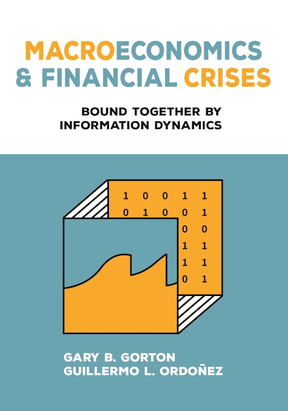
- Look Inside
- Request Exam Copy
- Download Cover
There are no bigger disruptions in the functioning of economies than financial crises. Yet prior to the crash of 2007–2008, macroeconomics incorporated financial crises simply as bad shocks, like earthquakes, failing to consider them as an intrinsic phenomenon of the evolution of macroeconomic variables, such as credit, investment, and productivity. Macroeconomics and Financial Crises rethinks how technological change, credit booms, and endogenous information production combine to generate financial crises as inherent and recurrent reactions to macroeconomic dynamics. Gary Gorton and Guillermo Ordoñez identify short-term debt, collateral, and information as common elements that are present in all financial crises. Short-term debt is a critical element for storing value over short periods without fear of loss, but there needs to be collateral backing the debt. Critically, the collateral should be such that no agent wants to produce information about its quality. The debt backed by such collateral is information-insensitive. Gorton and Ordoñez argue that, during a credit boom, as more and more firms get loans, the economy reaches a tipping point where information production becomes too tempting, disrupting short-term debt and cutting most firms out of the credit market. Showing how a financial crisis is an information event triggered by the dynamics of macroeconomic variables, Macroeconomics and Financial Crises provides new perspectives on the intricate relations between macroeconomics and financial crises.
“Economics has been treating financial crises as disruptive events beyond equilibrium explanation. Gorton and Ordoñez challenge this view by showing that crises are information events amenable to equilibrium analysis. This book advances our understanding of financial crises and shows, theoretically and empirically, how incorporating them can enrich macroeconomic analyses.”—Bengt Holmström, Massachusetts Institute of Technology
“This landmark graduate book provides a novel perspective on credit booms and financial crises centered around informational insensitivity, opacity, and liquidity of short-term debt. It is essential reading for anyone who wants to be on the cutting edge of the financial crisis research frontier.”—Markus K. Brunnermeier, coauthor of A Crash Course on Crises
“Through a collection of fascinating facts, narratives, and models, Gorton and Ordoñez synthesize and expand their decade-long research project on the key role played by collateral-quality information and credit in financial crises. It is now required reading in my financial crises course.”—Ricardo Caballero, Massachusetts Institute of Technology
“What happens when an asset that is widely accepted as collateral suddenly becomes suspect? Using a modern theory approach rooted in information and informed by history, Gorton and Ordoñez explore what causes, follows, and cures a financial crisis. A must-read for anyone seeking the frontier of research at the intersection of macroeconomics, banking, and finance.”—Laura L. Veldkamp, Columbia University, author of Information Choice in Macroeconomics and Finance
Stay connected for new books and special offers. Subscribe to receive a welcome discount for your next order.
- ebook & Audiobook Cart
Modeling Financial Crises
Pascal Paul
Download PDF (164 KB)
FRBSF Economic Letter 2019-08 | March 4, 2019
Research has revealed several facts about financial crises based on historical data. Crises are rare events that are associated with severe recessions that are typically deeper than normal recessions. They are usually preceded by a buildup of system imbalances, particularly a rapid increase of credit. Financial crises tend to occur after prolonged booms but do not necessarily result from large shocks. Recent work shows a novel way to replicate these facts in a standard macroeconomic model, which policymakers could use to gain insights to prevent future crises.
The 2007–09 financial crisis made it plain that, even for developed economies like the United States, severe financial disruptions can drag down a whole economy. The crisis and the slow recovery that followed have sparked an explosion of research that aims to account for the tight linkages between the financial sector and the macroeconomy. Such research is important to policymakers since it could help avert future crises or provide guidance to ameliorate their effects.
Financial crises are characterized by a sudden and widespread decline in asset values, a sharp deviation from normal financial market functioning, and a severe tightening of credit that leads to a contraction in economic activity. Before the 2007–09 crisis, the workhorse macroeconomic models used by many central banks around the world largely excluded financial institutions and, therefore, did not account for the possibility of such events. Over the past decade, many advances have addressed these shortcomings. However, up to this point, a common approach to integrate financial crises into macroeconomic models has not yet emerged.
In this Economic Letter , I argue for applying a useful guiding principle: models that researchers use to understand financial crises should be able to replicate stylized facts gathered from historical data. I focus on four important facts about crises. Matching these patterns within a single model is an important challenge for realistic macroeconomic models of financial crises. I outline recent work by Paul (2019) that aims to address this issue and presents a framework that is able to match key features of crises in the data.
Four facts about crises
Crises are rare events. On average, crises occur about every 25 years or even less frequently. In contrast, a new recession typically starts around every 8 years. This first fact already poses an immediate challenge when studying financial crises empirically. To obtain enough observations to study common patterns around crises, researchers need large data sets. That is, data sets have to cover many countries and reach back decades. Hence, research usually relies on historical sources and often involves tedious archive work.
Credit booms tend to precede crises. A wide range of historical studies have shown that financial crises are not entirely random events that are unrelated to macroeconomic conditions. By contrast, crises typically occur at the end of an expansion, after a prolonged buildup of macrofinancial imbalances.
One key determinant of crises that has emerged is aggregate credit issued to nonfinancial firms and households. For example, Schularick and Taylor (2012) found that aggregate credit growth is a reliable early-warning indicator. Figure 1 illustrates this pattern, showing the annual percentage change of credit in the years before and after crises based on data for 17 advanced economies from 1870 to 2013. In the run-up to a crisis, credit typically expands quickly, falls sharply around the outbreak, and remains depressed in the aftermath.
Financial crises are associated with severe recessions. Once a financial crisis breaks out, output typically declines more strongly than during a normal recession. Also, the fall in output is even stronger if the crisis is preceded by a buildup of credit, as found in Jordà, Schularick, and Taylor (2013). For example, GDP falls around 30–50% more during a typical financial crisis recession compared with a normal recession (Paul 2019). A potential explanation is that the availability of credit tightens around the outbreak of a crisis that affects economic activity, as Figure 1 shows.
Figure 1 Typical behavior of credit around financial crises
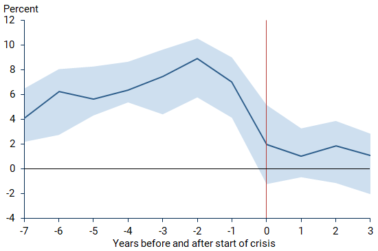
Note: Median (dark blue line) and 33rd and 66th percentile (shaded areas) of annual percentage change in credit; year zero (red line) denotes start of a crisis. See Paul (2019) for details.
The ultimate triggers of crises can be relatively small. Even though output falls sharply during a crisis, this may not simply be due to a large shock that has hit the economy. For example, Gorton and Ordonez (2014) argue that the losses from mortgage-backed securities in the 2007–09 financial crisis–which was the relevant shock for the financial sector around that time—were actually quite modest. The U.S. financial system may have been particularly vulnerable to small shocks around 2007, so a similar trigger at another time might not have resulted in such a large disruption to the financial system.
To sum up, crises display the following characteristics: they are rare events that are typically preceded by a buildup of credit, are associated with deeper recessions than normal, and are not necessarily triggered by large shocks. These empirical facts about crises pose challenges to macroeconomic models. Why does financial fragility build up in good times when credit expands? Also, what propagation mechanism turns shocks that are not particularly large into severe macroeconomic events?
A macroeconomic model with occasional financial crises
Folding these facts about financial crises into a macroeconomic model is an important challenge for researchers. The approach I describe here is based on Paul (2019), while Boissay, Collard, and Smets (2016) present an alternative framework that emphasizes a different set of financial market mechanisms. The model in Paul (2019) focuses on the interactions between households, banks, and nonfinancial firms. All three play a key role in the chain of financial intermediation. Households save by depositing funds in banks. In turn, banks redirect household savings to help finance business activity. Hence, in the model, banks stand in for the joint financial intermediation activities of the modern financial sector.
Next, imagine a scenario in which the economy is booming and businesses are particularly productive. During a boom, households receive additional income. However, they prefer to save part of it to smooth their consumption over time. In turn, banks convert the additional deposits into new lending to businesses. Hence, banks expand their balance sheets during prolonged booms. They increase both their assets through loans to businesses and their liabilities through increased household deposits. As in the data, banks also raise their leverage—that is, the ratio of liabilities to assets during prolonged expansions. However, by increasing their leverage during the boom, bank balance sheets also become more fragile since banks borrow more relative to the value of their assets. In this way, financial instability can build during good times when credit expands.
The boom turns into a bust when businesses become less productive and the economy slows down. During the slowdown, more businesses are unable to repay their loans, and their decision to default puts pressure on bank balance sheets. When banks’ assets fall in value due to the increased chance of default, then their leverage—the ratio of liabilities to assets—spikes up sharply.
The rise in leverage increases the risk that banks will not pay households back in full in case there is a run on the bank. To prevent runs and therefore bankruptcy, banks strongly cut back on their lending by liquidating outstanding loans inefficiently and reducing new lending. In this way, banks are able to generate additional liquidity that could be used to pay back deposits and therefore prevent households from running on banks. However, the early liquidation of loans and the subsequent ending of the underlying investment projects causes aggregate investment and output to drop sharply. Through this mechanism, the model turns moderate adverse shocks into large macroeconomic effects.
Simulations provide evidence that the model is able to match the four facts about crises. First, crises in the model occur as frequently as in the data. Second, a prolonged and credit-fueled boom characterizes the typical path leading to a crisis as illustrated in Figure 2, panel A. Third, the resulting crises are as severe as in the data. Fourth, crises are usually triggered by a relatively moderate adverse shock, but output still falls sharply due to the early liquidation of investment, as illustrated in Figure 2, panel B.
Figure 2 How do overall credit and output behave before and after financial crises?
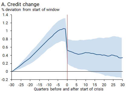
Note: Median (dark blue line) and 33rd and 66th percentiles (shaded areas) around start of financial crisis at quarter 0 (red lines). See Paul (2019) for details.
In addition, the mechanisms through which financial fragility builds up and a crisis materializes are empirically validated. First, the leveraging behavior of banks that explains why financial instability increases in good times is supported by the data. Leverage of U.S. financial intermediaries valued at market prices is mildly procyclical—that is, it is positively correlated with economic activity—in the model and in the data.
Second, recent evidence by Chodorow-Reich and Falato (2017) shows that overall credit during the 2007–09 financial crisis contracted primarily because banks renegotiated the loan terms or accelerated repayment on existing credit, as is the case in the model I have described. Thus, taken together, the model is able to match key characteristics of financial crises in the data, and the mechanisms through which that is achieved are empirically supported.
This Economic Letter describes four empirical facts about financial crises: (1) crises are rare, (2) they occur out of credit booms, (3) they are severe macroeconomic events, and (4) they are not necessarily the result of large shocks. Macroeconomic models of financial crises should replicate all of these features to accurately reflect what occurs around a typical crisis. The model in Paul (2019) reproduces these real-world regularities and illustrates how standard macroeconomic models can be extended to incorporate occasional financial crises. Such a framework provides a suitable laboratory for additional research that can help policymakers understand how to reduce the likelihood and the severity of future crises.
Pascal Paul is an economist in the Economic Research Department of the Federal Reserve Bank of San Francisco.
Boissay, Frédéric, Fabrice Collard, and Frank Smets. 2016. “Booms and Banking Crises.” Journal of Political Economy 124(2), pp. 489–538.
Chodorow-Reich, G. and Antonio Falato. 2017. “The Loan Covenant Channel: How Bank Health Transmits to the Real Economy.” NBER Working Paper 23879.
Gorton, G., and Guillermo Ordoñez. 2014. “Collateral Crises.” American Economic Review 104(2), pp. 343–378.
Jordà, Òscar, Moritz Schularick, and Alan M. Taylor. 2013. “When Credit Bites Back.” Journal of Money, Credit, and Banking 45(s2), pp. 3–28.
Paul, Pascal. 2019. “A Macroeconomic Model with Occasional Financial Crises.” FRBSF Working Paper 2017-22.
Schularick, Moritz, and Alan M. Taylor. 2012. “Credit Booms Gone Bust: Monetary Policy, Leverage Cycles, and Financial Crises, 1870–2008.” American Economic Review 102(2), pp. 1,029–61.
Opinions expressed in FRBSF Economic Letter do not necessarily reflect the views of the management of the Federal Reserve Bank of San Francisco or of the Board of Governors of the Federal Reserve System. This publication is edited by Anita Todd and Karen Barnes. Permission to reprint portions of articles or whole articles must be obtained in writing. Please send editorial comments and requests for reprint permission to [email protected]
Program on Financial Stability Resource Library
Program on financial stability, resource library, us government crisis response.
The Global Financial Crisis (GFC) of 2007-2009 was the most significant financial crisis to hit the US economy since the Great Depression. The US government’s response to the GFC was multifaceted and encompassed many different policy interventions involving multiple government agencies and various economic sectors. While the initial response relied primarily on traditional methods and authority, later government actions utilized more unconventional approaches. This research guide highlights some of the significant actions taken by the Federal Reserve, the Treasury, the Federal Deposit Insurance Corporation (FDIC) and other government entities to stabilize the financial system and the economy during the period of 2007-2010.
The following two charts from the Treasury’s publication The Financial Crisis Five Years Later: Response, Reform, and Progress In Charts and the Brookings-YPFS publication Charting the Financial Crisis provide visual introductions to the government’s response. Chart 1 highlights the breadth of efforts undertaken and the different sectors served, and Chart 2 shows how the nature of the responses changed as the crisis evolved over time.

|
| |
| . YPFS and the Brookings Institution, Hutchins Center on Fiscal and Monetary Policy (2018) | |
| (including the Fed’s Financial Crisis Financing Programs)
| s |
| to investigate the causes of the crisis. The commission held hearings, gathered data and information and delved into the details. In February 2011, it issued its final report, which is considered the definitive report on the crisis. was enacted on July 21, 2010, in response to the crisis. It was the most sweeping amendment to US financial regulatory system since the Depression era. The act revamped the system, eliminating the Office of thrift Supervision, assigning new duties to the FDIC and Federal reserve and creating a new consumer agency, the Consumer Financial Protection Bureau. and the . The Federal Reserve received new authority to regulate systemically important institutions (SIFIS) that were to be designated by the FSOC; and these could be nonbanks. To handle the liquidation of large companies, Dodd-Frank required SIFIs to submit resolution plans (living wills”) to the government and created the Orderly Liquidation Authority pursuant to which the FDIC, with its long history of resolving banks, would step in to resolve failing SIFIs.
| |
Copyright 2019 Yale Program on Financial Stability
- Today's Paper
- Markets Data
- Interest rates
Debt and deficits may cause financial crisis, RBA research boss warns

Subscribe to gift this article
Gift 5 articles to anyone you choose each month when you subscribe.
Already a subscriber? Login
Persistent budget deficits may cause the next global financial crisis, as investors decide government debt is no longer a safe asset, badly damaging banks’ balance sheets, RBA research boss John Simon has warned in his final remarks.
Dr Simon said the biggest medium-term risk to global financial stability was what he termed the “bank-sovereign nexus”, where investors abandoned the widely held assumption that government debt was safe, causing a financial market meltdown.
Introducing your Newsfeed
Follow the topics, people and companies that matter to you.
Latest In Economy
Fetching latest articles
Most Viewed In Policy
Fincialization and Corporate Investment in Korea after the Asian Financial Crisis
- Wright State University
Research output : Other contribution
| Original language | American English |
|---|---|
| State | Published - Nov 6 2011 |
Disciplines
- Social and Behavioral Sciences
Access to Document
- http://www.economicpolicyresearch.org/images/docs/SCEPA_blog/SCEPA_news/NSSR_UMass_Workshop_2011_Program_v4.pdf
Other files and links
- Link to repository
- Link to publication
T1 - Fincialization and Corporate Investment in Korea after the Asian Financial Crisis
AU - Shin, Hee-Young
PY - 2011/11/6
Y1 - 2011/11/6
UR - https://corescholar.libraries.wright.edu/econ/209
UR - http://www.economicpolicyresearch.org/images/docs/SCEPA_blog/SCEPA_news/NSSR_UMass_Workshop_2011_Program_v4.pdf
M3 - Other contribution
Money blog: Blue Light discount anger as teachers added; pound falls for four straight weeks
Welcome to the Money blog, your place for personal finance and consumer news/tips. Today's posts include four weeks of falls for the pound and this week's Money Problem - you can submit yours (remember to leave contact details or we can't look into it) below.
Monday 12 August 2024 19:13, UK
- Pound falls for four straight weeks - here's what it means
- Blue Light discount for teachers prompts backlash - but poll suggests public support move
- Unusually cheap package holidays on offer - but travel writer dismisses Russia theory
- Compensation for poor water service to double
- Revolution Bar's restructuring plan approved by court
Essential reads
- Money Problem : 'I cancelled swimming lessons and they are keeping my money - do I have any rights?'
- Is this the end of the British pub?
- The rise of 'doom spending' - what it is and how to stop
- Where kids can eat for free or cheap
- Best of the Money blog - an archive of features
Ask a question or make a comment
Heathrow says a drop in passenger numbers is down to a government scheme that charges non-visa connecting travellers £10 to pass through the airport .
It said the electronic travel authorisation (ETA) had been "devastating for our hub competitiveness" - accounting for a 90,000 drop in passengers.
The chairman of Asda says he is "embarrassed" by the supermarket's recent decline.
The retail giant reported a 2.1% drop in like-for-like sales in the first half of the year.
Asda has also lost market share since it was acquired by the Issa brothers in 2021.
Lord Rose told The Telegraph he was "slightly embarrassed" and did not like "being second, third or fourth".
Card Factory has teamed up with food delivery app Just Eat to offer customers the chance to get greetings cards delivered to their door as quickly as a takeaway.
The partnership is live in 19 stores across the UK, including Liverpool, Manchester and London, and is set to be extended.
Rioting caused sales to plummet as much as 40% in areas where rallies, protests and riots were rumoured to take place last Wednesday, according to a hospitality association.
Businesses reported footfall was down by as much as 75% in some locations, while sales fell by 10% across the country, UKHospitality said.
Shops closed down, events were cancelled in city centres, and customers stayed away, working from home and cancelling day trips to coastal towns.
"These figures are startling and show the enormous impact the riots, and threat of further disorder, have had on our high streets and communities," said Kate Nicholls, chief executive of UKHospitality.
"Bustling, vibrant city centres were turned into ghost towns as the public stayed at home and businesses shut."
A flooring company which trades out of John Lewis has collapsed into administration, resulting in the loss of around 200 jobs.
The Floor Room, a sister firm of Carpetright, closed concessions in 34 John Lewis shops on Friday and appointed administrators PwC.
A message on the company's now-closed website confirms the company has ceased trading and will not complete outstanding orders.
The accounting firm said management at the collapsed company had "exhausted options to secure further funding or a potential sale" prior to calling in administrators.
Some 201 employees are losing their jobs as a result of the move.
What are your rights?
If you've paid for an unfulfilled order, or want to return an item, a lack of shops mean you have to file a claim with administrators PwC to join a list of creditors owed money – but there's no guarantee you'll get your money back.
Credits and debits
You can file a claim with your debit or credit card provider to recover lost funds:
- Credit card: If you bought any single item costing between £100-£30,000 and paid on a credit card, the card firm is liable if something goes wrong. If any purchase was less than £100, you may still be able to get your money back via chargeback;
- Debit card: Under chargeback, your bank can try to get your money back from The Floor Room's bank. However, be aware that this is not a legal requirement and it can later be disputed and recalled back.
The battle to bring down inflation is not over, a Bank of England ratesetter has warned, as she urges Britons not to be "seduced" into thinking the country is out of the woods.
Catherine Mann, an external member of the BoE's Monetary Policy Committee (MPC), said she was still worried inflation could rise again despite it coming down to the 2% target.
She told the Financial Times that pay growth (currently way above inflation at 5.7% with updated figures due this week) could pose a problem, with companies still expected to make increases to wages and prices.
"That says to me right now I'm looking at a problem for next year," she told the newspaper.
"There is an upwards ratchet to both the wage-setting process and the price process and... it may well be structural, having been created during this period of very high inflation over the last couple of years," she added.
"That ratchet up will take a long time to erode away."
Ms Mann was one of four members of the nine-strong MPC who voted to keep interest rates at 5.25% last month - and it sounds like she isn't likely to shift position ahead of September's rate decision.
A revamped Waitrose store in north London will reopen soon with fancy new features - including a parmesan bay - as the upmarket grocer unveils its new store concept.
The John Barnes store on Finchley Road has undergone a major six-week refurbishment and is set to reopen on 21 August.
According to Retail Gazette , the store will have a number of new features including a new look and feel bakery, an in-branch baguette station and even a "dedicated parmesan bay".
The supermarket chain said it would also be the first to have a hot wok counter serving ready-to-go meals.
The John Barnes site is being used as a tester for its new concepts, it added.
On Friday we reported on teachers being given access to the Blue Light discount scheme - which appeared to elicit a backlash on social media...
We had scores of reader comments - all but one onside with the backlash (see below).
This morning, we asked our followers on LinkedIn for their view. The poll is still active , but the results so far suggest a level of support for teachers...
The discrepancy between the way people are voting on LinkedIn and the comments here in the Money blog could be interpreted in several ways. Sky News could be followed by different demographics on the two platforms, or perhaps it is that those who feel most angry at something are far more likely to leave a comment.
Whatever the explanation, here's a selection of comments that sum up the general feeling in our inbox...
If you change it to key workers then you would have to open it to shop workers, waste disposal workers, plumbers and electricians. Dave
Blue light is in the name. Shift workers who work long unsociable hours in a responsive role. Pure greed by the administrators of the scheme. Shawhome
How long have teachers been an emergency service? I don't remember them being on the front line during COVID. I haven't seen them during the riots. Swiftrider
Teaching is NOT an emergency service. I'm a carer to a child and get paid peanuts, no Blue Light card for me. Joseph Morgan
As a gas emergency engineer who is safeguarding life and property who has an hour from the reported time to get to the gas escape... we get there quicker than the ambulance service and occasionally police but we can't get a Blue Light card. Just wondering why? Senseirick
Teachers do a good job, but to actually class them as blue light is shameful. When was the last time a teacher went home and wept after loosing a patient or had to stand in a line behind a shield getting bricked by a mob? Or being shot at in a foreign land? Ianstu
Farmers feed the nation, when will they be entitled to a Blue Light Card? Greatauntbleach
An emergency service is available 24 hours a day. 365 days per year. Teachers are not. They are valuable in society, absolutely, but they are not an emergency service with a blue light. Joanna Clark
Wow. 30 years as a prison officer, working very unsociable hours, getting abused, assaulted. Nowhere near the amount of time off that teachers get. Police, NHS, armed services deserve this, not teachers. Noslop17
We did have one correspondent backing teachers - and of course our inbox is still open if you want to share your view...
Good to see teachers getting the Blue Light card as an essential service for children's future - and also what about teaching assistants, lunch supervision and school club staff. If schools shut, the whole country is affected, especially parents not working, during strikes or bad weather. Southwest lady
Blue Light hits back
Blue Light Card hit back on Friday, saying: "Teachers are not just educators; they are mentors, guides and inspirations that are helping shape the future for our children. They are fully deserving members of our blue light community."
What kind of offers can a Blue Light card get you?
There's too many to list but among the offers is 12% off at Fenty Beauty and 15% off at Bose.
Users can also get a £30 gift card if they spend more than £1,000 at British Airways or a £110 voucher if they sell their car via Carwow.
Or if getting fit is more your thing, you can get 50% off an annual subscription to the Body Coach.
The pound last week completed its fourth consecutive weekly fall against the US dollar – something that will have worried British tourists heading to the US this summer.
Since hitting a high for the year of $1.3044 on 17 July, sterling slipped to a low of $1.2662 last Thursday, but has since rallied to as much as $1.2782 this morning.
Against the euro, the pound has traded similarly. It hit a peak of €1.1927 on 17 July but then fell to as low as €1.1584 last Thursday before rallying to as much as €1.1703 today.
The reason for these reverses is pretty straightforward.
Since the Bank of England cut interest rates on 1 August, for the first time since 2020, the markets have started to price in the prospect of at least one further interest rate cut between now and the end of the year. That obviously has implications for the pound.
It is important to put this recent weakness into context.
Until last month, sterling had been one of the best performing currencies globally so far this year, hitting its highest level for a year last month. That reflected the strength of the UK economy which, during the first half of this year, had been the best performing economy in the G7.
So the recent weakness, such as it is, is really not that remarkable – and analysts still think, all other things being equal, that the "bull case" for sterling remains intact.
By Sarah Taaffe-Maguire , business reporter
It looks set to be a quieter week on the markets compared with last week which started with a global market sell-off prompted by fears of the US economy being in recession and worries of tech company performance.
But there'll be plenty of new information for investors to chew over as latest inflation, economic growth and employment data is released over the coming four days.
As stock market values rebounded, so too did the benchmark oil price. A barrel of Brent crude now costs $80.09, greater than at any point last week, spelling more expensive fuel refilling for motorists.
The pound has come off the highs against the dollar seen earlier in the summer. One pound now buys $1.2768. Similarly it is weaker against the euro with £1 equal to €1.1689.
Both of the UK's major stock market indexes started the week up. The Financial Times Stock Exchange (FTSE) 100 index of most valuable companies on the London Stock Exchange rose 0.57%, while the larger and more UK-based FTSE 250 index was up 0.34%.
Compensation for customers experiencing poor service from their water providers is to more than double under new government proposals.
The plans will see compensation paid in more circumstances - including automatic payments for people who are told to boil their water in certain areas or when firms miss scheduled appointments.
Earlier this year, residents in the Devon town of Brixham were told to boil their water for eight weeks after the local supply was hit by a parasite outbreak.
People affected by an incorrect notice telling them their supply will be interrupted could also see their payout rise from £20 to £50, while those being reimbursed for internal flooding from sewers could see a maximum payment of £2,000 rather than the current £1,000.
It's hoped the proposals - which are now subject to an eight-week consultation - will "turn the tide on the destruction of our waterways", Environment Secretary Steve Reed said.
Every Monday the Money team answers your Money Problems or consumer disputes. Find out how to submit yours at the bottom of this post. Today's question is...
I had a frustrating issue with my kids' swimming lessons. We had to pay in advance, but when your child says they don't want to go any more, that's it, they don't go. I asked the club if we can get a refund for the remaining month that they won't attend but the club just say, 'Your child is eligible to come for the next four weeks.' Doesn’t seem quite fair. Richard Wallace, West Sussex
Hi Richard, we can understand why this doesn't seem fair. You are trying to cancel with what sounds like a reasonable amount of notice and yet you're getting nowhere.
This is a common occurrence and many readers will have been in a similar situation.
The law says that you can cancel a service you've booked online or by phone (or by mail order) within a 14-day cooling-off period.
This might be a cleaner or electrician or surveyor.
This cooling-off period also applies if a business approached you away from their premises if the service costs £42 or more.
The bad news in your case, though, is that the above does not apply to accommodation, delivery services, vehicle hire or - and this is the relevant one here - leisure or catering activities for specific dates.
In these cases, you'd be relying on their being a generous cancellation policy - so you should check their T&Cs.
It might not be a dead end, though.
You should try to negotiate with them - it's generally accepted this can be done when a cancellation charge seems unfair or when a business is withholding more money than needed to cover their losses.
Ask them if they're part of a trade association, which you could request help from in negotiating.
Beyond this, they might be a member of an alternative dispute resolution (ADR) scheme. Again, it's worth asking. If not, you could choose a Trading Standards-approved ADR scheme yourself to approach.
We suspect the sums involved here are not big enough for you to consider going to court - but if this was an avenue you wanted to explore here or in future, keep records of all the above steps.
As a last resort you can take your case to the Small Claims Court in England and Wales - or use the respective legal routes in Scotland and Northern Ireland .
Further help
The Citizens Advice consumer helpline is a great resource - it's 0808 223 1133. You can also use an online form .
If you're in Northern Ireland, contact Consumerline .
This feature is not intended as financial advice - the aim is to give an overview of the things you should think about. Submit your dilemma or consumer dispute via:
- The form above - you need to leave a phone number or email address so we can contact you for further details;
- Email [email protected] with the subject line "Money blog";
- WhatsApp us here.
Be the first to get Breaking News
Install the Sky News app for free

COMMENTS
by Robin Greenwood, Samuel G. Hanson, Andrei Shleifer, and Jakob Ahm Sørensen. One central issue in the study of macroeconomic stability is financial crisis predictability. This paper estimates the probability of financial crises as a function of past credit and asset price growth. 23 Apr 2020. Research & Ideas.
The "Ten Years After" Brief contains summaries of research articles and central banker discussions from the "2008 Financial Crisis: A Ten-Year Review" conference that took place in November 2018 in New York City. The full versions of the articles were published by the Annual Review of Financial Economics, and actual live conference ...
Research Department Financial Crises: Explanations, Types, and Implications Prepared by Stijn Claessens and M. Ayhan Kose1 January 2013 Abstract This paper reviews the literature on financial crises focusing on three specific aspects. First, what are the main factors explaining financial crises? Since many theories on the
The Financial Crisis: Toward an Explanation and Policy Response. by Aaron Steelman and John A.Weinberg. in Federal Reserve Bank of Richmond Annual Report 2008, April 2009. The essay is divided into the four sections. First, what has happened in the financial markets.
Long-run historical data for advanced economies provide evidence to help policymakers understand specific conditions that typically lead up to financial crises. Recent research finds that rapid growth in the top income share and prolonged low labor productivity growth are robust predictors of crises. Moreover, if crises are preceded by these developments, then the subsequent recoveries are ...
Financial crises are a centuries-old phenomena (see Reinhart and Rogoff 2008, 2009, 2014), and there is a substantial literature on the subject (e.g., ... Most research attention has been focused on the optimal design of regulations, but we need more research on the kinds of regulatory institutions needed to implement simple and effective ...
DOI 10.3386/w32213. Issue Date March 2024. The high social costs of financial crises imply that economists, policymakers, businesses, and households have a tremendous incentive to understand, and try to prevent them. And yet, so far we have failed to learn how to avoid them. In this article, we take a novel approach to studying financial crises.
The paper focuses on the main theoretical and empirical explanations of four types of financial crises—currency crises, sudden stops, debt crises, and banking crises—and presents a survey of the literature that attempts to identify these episodes. ... Working Papers describe research in progress by the author(s) and are published to elicit ...
Financial crises: A survey Amir Sufi and Alan M. Taylor August 2021. JEL No. E32,E44,E7,G01,G10,N20ABSTRACTFinancial crises have large deleterious effects on economic activity, and as such have be. n the focus of a large body of research. This study surveys the existing literature on financial crises, exploring how crises are measured, whether ...
Amir Sufi & Alan M. Taylor. Financial crises have large deleterious effects on economic activity, and as such have been the focus of a large body of research. This study surveys the existing literature on financial crises, exploring how crises are measured, whether they are predictable, and why they are associated with economic contractions.
The massive and multifaceted policy responses to the financial crisis and Great Recession — ranging from traditional fiscal stimulus to tools that policymakers invented on the fly — dramatically reduced the severity and length of the meltdown that began in 2008; its effects on jobs, unemployment, and budget deficits; and its lasting impact on today's economy.
14 crises seem highly predictable using a simple indicator variable that switches on when credit growth and asset price growth are jointly elevated. While the probability of a crisis following the -zone is high, the within-country. R forecasting R. 2. is more modest. For example, at a 3 -year horizon, R.
42 Financial Crises: Explanations, Types, and Implications. including the appreciation of the real exchange rate (relative to trend), a banking. crisis, a decline in equity prices, a decline in ...
In the early 1930s, he concludes, policy errors by governments and central banks turned a financial crisis into a global economic disaster. In 2008 the financial shock was at least as big, but the ...
Financial Crisis: A financial crisis is a situation in which the value of financial institutions or assets drops rapidly. A financial crisis is often associated with a panic or a run on the banks ...
It is essential reading for anyone who wants to be on the cutting edge of the financial crisis research frontier."—Markus K. Brunnermeier, coauthor of A Crash Course on Crises "Through a collection of fascinating facts, narratives, and models, Gorton and Ordoñez synthesize and expand their decade-long research project on the key role ...
Research has revealed several facts about financial crises based on historical data. Crises are rare events that are associated with severe recessions that are typically deeper than normal recessions. They are usually preceded by a buildup of system imbalances, particularly a rapid increase of credit. Financial crises tend to occur after prolonged booms but do not necessarily result from large ...
John B. Taylor* November 2008. Abstract: This paper is an empirical investigation of the role of government actions and interventions in the financial crisis that flared up in August 2007. It integrates and summarizes several ongoing empirical research projects with the aim of learning from past policy and thereby improving future policy.
Research Associate, YPFS, Yale School of Management. 5 . Research Scholar and Director of Research, YPFS, Yale School of Management. ... Financial Crisis of 2007-2009 (GFC), few countries had resolution regimes that allowed authorities to intervene in failing financial firms. When confronted with the failure of a large
A financial crisis is any of a broad variety of situations in which some financial assets suddenly lose a large part of their nominal value. ... Empirical and econometric research continues especially in the world systems theory and in the debate about Nikolai Kondratiev and the so-called 50-years Kondratiev waves.
303. 2008 Financial Crisis: Causes and Costs. Jiaming Cui *. School of Finance and Investment, Guangdong University of Finance, Guangzhou, China. *Corresponding author: [email protected] ...
US Government Crisis Response. The Global Financial Crisis (GFC) of 2007-2009 was the most significant financial crisis to hit the US economy since the Great Depression. The US government's response to the GFC was multifaceted and encompassed many different policy interventions involving multiple government agencies and various economic sectors.
consequences of financial crises and policy responses to them. Although there is a rich literature on financial crises, there has been no publication since the recent financial crisis providing in one place a broad overview of this research and distilling its policy lessons. The book fills this critical gap.
and the probability of financial crises; and a set of case studies of rapid debt buildup that ended in crises. The paper reports four main results. First, episodes of debt accumulation are common, with more than 500 episodes occurring since 1970. Second, around half of these episodes were associated with financial crises which typically had
Bin Li obtained her PhD in Economics with a thesis focused on the topic of central bank's anti-crisis policies. Currently, she is Assistant Research Fellow at Academy of Marxism, Chinese Academy of Social Sciences. Her main research interests are in the fields of political economy, fiscal crises, monetary policy, and other related areas.
Persistent budget deficits may cause the next global financial crisis, as investors decide government debt is no longer a safe asset, badly damaging banks' balance sheets, RBA research boss John ...
literature and future research directions. ... Financial crises are often preceded by asset and credit booms that eventually turn into busts. Many theories focusing on the sources of crises have recognized the importance of booms in asset and credit markets. However, explaining why asset price bubbles or credit booms are ...
TY - GEN. T1 - Fincialization and Corporate Investment in Korea after the Asian Financial Crisis. AU - Shin, Hee-Young. PY - 2011/11/6. Y1 - 2011/11/6
The Financial Times Stock Exchange (FTSE) 100 index of most valuable companies on the London Stock Exchange rose 0.57%, while the larger and more UK-based FTSE 250 index was up 0.34%.
The industry's capacity utilization has fallen to about 78 percent, German research institute Ifo said, nine percentage points below the long-term average, as automakers including VW reduce output.