example of case study about climate change

11 min read

Seven case studies in carbon and climate

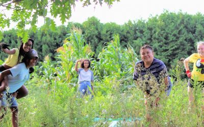
Every part of the mosaic of Earth's surface — ocean and land, Arctic and tropics, forest and grassland — absorbs and releases carbon in a different way. Wild-card events such as massive wildfires and drought complicate the global picture even more. To better predict future climate, we need to understand how Earth's ecosystems will change as the climate warms and how extreme events will shape and interact with the future environment. Here are seven pressing concerns.

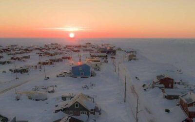
The Far North is warming twice as fast as the rest of Earth, on average. With a 5-year Arctic airborne observing campaign just wrapping up and a 10-year campaign just starting that will integrate airborne, satellite and surface measurements, NASA is using unprecedented resources to discover how the drastic changes in Arctic carbon are likely to influence our climatic future.

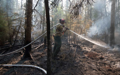
Wildfires have become common in the North. Because firefighting is so difficult in remote areas, many of these fires burn unchecked for months, throwing huge plumes of carbon into the atmosphere. A recent report found a nearly 10-fold increase in the number of large fires in the Arctic region over the last 50 years, and the total area burned by fires is increasing annually.

Organic carbon from plant and animal remains is preserved for millennia in frozen Arctic soil, too cold to decompose. Arctic soils known as permafrost contain more carbon than there is in Earth's atmosphere today. As the frozen landscape continues to thaw, the likelihood increases that not only fires but decomposition will create Arctic atmospheric emissions rivaling those of fossil fuels. The chemical form these emissions take — carbon dioxide or methane — will make a big difference in how much greenhouse warming they create.

Initial results from NASA's Carbon in Arctic Reservoirs Vulnerability Experiment (CARVE) airborne campaign have allayed concerns that large bursts of methane, a more potent greenhouse gas, are already being released from thawing Arctic soils. CARVE principal investigator Charles Miller of NASA's Jet Propulsion Laboratory (JPL), Pasadena, California, is looking forward to NASA's ABoVE field campaign (Arctic Boreal Vulnerability Experiment) to gain more insight. "CARVE just scratched the surface, compared to what ABoVE will do," Miller said.

Methane is the Billy the Kid of carbon-containing greenhouse gases: it does a lot of damage in a short life. There's much less of it in Earth's atmosphere than there is carbon dioxide, but molecule for molecule, it causes far more greenhouse warming than CO 2 does over its average 10-year life span in the atmosphere.

Methane is produced by bacteria that decompose organic material in damp places with little or no oxygen, such as freshwater marshes and the stomachs of cows. Currently, over half of atmospheric methane comes from human-related sources, such as livestock, rice farming, landfills and leaks of natural gas. Natural sources include termites and wetlands. Because of increasing human sources, the atmospheric concentration of methane has doubled in the last 200 years to a level not seen on our planet for 650,000 years.

Locating and measuring human emissions of methane are significant challenges. NASA's Carbon Monitoring System is funding several projects testing new technologies and techniques to improve our ability to monitor the colorless gas and help decision makers pinpoint sources of emissions. One project, led by Daniel Jacob of Harvard University, used satellite observations of methane to infer emissions over North America. The research found that human methane emissions in eastern Texas were 50 to 100 percent higher than previous estimates. "This study shows the potential of satellite observations to assess how methane emissions are changing," said Kevin Bowman, a JPL research scientist who was a coauthor of the study.

Tropical forests

Tropical forests are carbon storage heavyweights. The Amazon in South America alone absorbs a quarter of all carbon dioxide that ends up on land. Forests in Asia and Africa also do their part in "breathing in" as much carbon dioxide as possible and using it to grow.

However, there is evidence that tropical forests may be reaching some kind of limit to growth. While growth rates in temperate and boreal forests continue to increase, trees in the Amazon have been growing more slowly in recent years. They've also been dying sooner. That's partly because the forest was stressed by two severe droughts in 2005 and 2010 — so severe that the Amazon emitted more carbon overall than it absorbed during those years, due to increased fires and reduced growth. Those unprecedented droughts may have been only a foretaste of what is ahead, because models predict that droughts will increase in frequency and severity in the future.

In the past 40-50 years, the greatest threat to tropical rainforests has been not climate but humans, and here the news from the Amazon is better. Brazil has reduced Amazon deforestation in its territory by 60 to 70 percent since 2004, despite troubling increases in the last three years. According to Doug Morton, a scientist at NASA's Goddard Space Flight Center in Greenbelt, Maryland, further reductions may not make a marked difference in the global carbon budget. "No one wants to abandon efforts to preserve and protect the tropical forests," he said. "But doing that with the expectation that [it] is a meaningful way to address global greenhouse gas emissions has become less defensible."

In the last few years, Brazil's progress has left Indonesia the distinction of being the nation with the highest deforestation rate and also with the largest overall area of forest cleared in the world. Although Indonesia's forests are only a quarter to a fifth the extent of the Amazon, fires there emit massive amounts of carbon, because about half of the Indonesian forests grow on carbon-rich peat. A recent study estimated that this fall, daily greenhouse gas emissions from recent Indonesian fires regularly surpassed daily emissions from the entire United States.

Wildfires are natural and necessary for some forest ecosystems, keeping them healthy by fertilizing soil, clearing ground for young plants, and allowing species to germinate and reproduce. Like the carbon cycle itself, fires are being pushed out of their normal roles by climate change. Shorter winters and higher temperatures during the other seasons lead to drier vegetation and soils. Globally, fire seasons are almost 20 percent longer today, on average, than they were 35 years ago.

Currently, wildfires are estimated to spew 2 to 4 billion tons of carbon into the atmosphere each year on average — about half as much as is emitted by fossil fuel burning. Large as that number is, it's just the beginning of the impact of fires on the carbon cycle. As a burned forest regrows, decades will pass before it reaches its former levels of carbon absorption. If the area is cleared for agriculture, the croplands will never absorb as much carbon as the forest did.

As atmospheric carbon dioxide continues to increase and global temperatures warm, climate models show the threat of wildfires increasing throughout this century. In Earth's more arid regions like the U.S. West, rising temperatures will continue to dry out vegetation so fires start and burn more easily. In Arctic and boreal ecosystems, intense wildfires are burning not just the trees, but also the carbon-rich soil itself, accelerating the thaw of permafrost, and dumping even more carbon dioxide and methane into the atmosphere.

North American forests

With decades of Landsat satellite imagery at their fingertips, researchers can track changes to North American forests since the mid-1980s. A warming climate is making its presence known.

Through the North American Forest Dynamics project, and a dataset based on Landsat imagery released this earlier this month, researchers can track where tree cover is disappearing through logging, wildfires, windstorms, insect outbreaks, drought, mountaintop mining, and people clearing land for development and agriculture. Equally, they can see where forests are growing back over past logging projects, abandoned croplands and other previously disturbed areas.

"One takeaway from the project is how active U.S. forests are, and how young American forests are," said Jeff Masek of Goddard, one of the project’s principal investigators along with researchers from the University of Maryland and the U.S. Forest Service. In the Southeast, fast-growing tree farms illustrate a human influence on the forest life cycle. In the West, however, much of the forest disturbance is directly or indirectly tied to climate. Wildfires stretched across more acres in Alaska this year than they have in any other year in the satellite record. Insects and drought have turned green forests brown in the Rocky Mountains. In the Southwest, pinyon-juniper forests have died back due to drought.

Scientists are studying North American forests and the carbon they store with other remote sensing instruments. With radars and lidars, which measure height of vegetation from satellite or airborne platforms, they can calculate how much biomass — the total amount of plant material, like trunks, stems and leaves — these forests contain. Then, models looking at how fast forests are growing or shrinking can calculate carbon uptake and release into the atmosphere. An instrument planned to fly on the International Space Station (ISS), called the Global Ecosystem Dynamics Investigation (GEDI) lidar, will measure tree height from orbit, and a second ISS mission called the Ecosystem Spaceborne Thermal Radiometer Experiment on Space Station (ECOSTRESS) will monitor how forests are using water, an indicator of their carbon uptake during growth. Two other upcoming radar satellite missions (the NASA-ISRO SAR radar, or NISAR, and the European Space Agency’s BIOMASS radar) will provide even more complementary, comprehensive information on vegetation.

Ocean carbon absorption

When carbon-dioxide-rich air meets seawater containing less carbon dioxide, the greenhouse gas diffuses from the atmosphere into the ocean as irresistibly as a ball rolls downhill. Today, about a quarter of human-produced carbon dioxide emissions get absorbed into the ocean. Once the carbon is in the water, it can stay there for hundreds of years.

Warm, CO 2 -rich surface water flows in ocean currents to colder parts of the globe, releasing its heat along the way. In the polar regions, the now-cool water sinks several miles deep, carrying its carbon burden to the depths. Eventually, that same water wells up far away and returns carbon to the surface; but the entire trip is thought to take about a thousand years. In other words, water upwelling today dates from the Middle Ages – long before fossil fuel emissions.

That's good for the atmosphere, but the ocean pays a heavy price for absorbing so much carbon: acidification. Carbon dioxide reacts chemically with seawater to make the water more acidic. This fundamental change threatens many marine creatures. The chain of chemical reactions ends up reducing the amount of a particular form of carbon — the carbonate ion — that these organisms need to make shells and skeletons. Dubbed the “other carbon dioxide problem,” ocean acidification has potential impacts on millions of people who depend on the ocean for food and resources.

Phytoplankton

Microscopic, aquatic plants called phytoplankton are another way that ocean ecosystems absorb carbon dioxide emissions. Phytoplankton float with currents, consuming carbon dioxide as they grow. They are at the base of the ocean's food chain, eaten by tiny animals called zooplankton that are then consumed by larger species. When phytoplankton and zooplankton die, they may sink to the ocean floor, taking the carbon stored in their bodies with them.

Satellite instruments like the Moderate resolution Imaging Spectroradiometer (MODIS) on NASA's Terra and Aqua let us observe ocean color, which researchers can use to estimate abundance — more green equals more phytoplankton. But not all phytoplankton are equal. Some bigger species, like diatoms, need more nutrients in the surface waters. The bigger species also are generally heavier so more readily sink to the ocean floor.

As ocean currents change, however, the layers of surface water that have the right mix of sunlight, temperature and nutrients for phytoplankton to thrive are changing as well. “In the Northern Hemisphere, there’s a declining trend in phytoplankton,” said Cecile Rousseaux, an oceanographer with the Global Modeling and Assimilation Office at Goddard. She used models to determine that the decline at the highest latitudes was due to a decrease in abundance of diatoms. One future mission, the Pre-Aerosol, Clouds, and ocean Ecosystem (PACE) satellite, will use instruments designed to see shades of color in the ocean — and through that, allow scientists to better quantify different phytoplankton species.

In the Arctic, however, phytoplankton may be increasing due to climate change. The NASA-sponsored Impacts of Climate on the Eco-Systems and Chemistry of the Arctic Pacific Environment (ICESCAPE) expedition on a U.S. Coast Guard icebreaker in 2010 and 2011 found unprecedented phytoplankton blooms under about three feet (a meter) of sea ice off Alaska. Scientists think this unusually thin ice allows sunlight to filter down to the water, catalyzing plant blooms where they had never been observed before.

Related Terms

• Carbon Cycle

Explore More

As the Arctic Warms, Its Waters Are Emitting Carbon

Runoff from one of North America’s largest rivers is driving intense carbon dioxide emissions in the Arctic Ocean. When it comes to influencing climate change, the world’s smallest ocean punches above its weight. It’s been estimated that the cold waters of the Arctic absorb as much as 180 million metric tons of carbon per year […]

Peter Griffith: Diving Into Carbon Cycle Science

Dr. Peter Griffith serves as the director of NASA’s Carbon Cycle and Ecosystems Office at NASA’s Goddard Space Flight Center. Dr. Griffith’s scientific journey began by swimming in lakes as a child, then to scuba diving with the Smithsonian Institution, and now he studies Earth’s changing climate with NASA.

NASA Flights Link Methane Plumes to Tundra Fires in Western Alaska

Methane ‘hot spots’ in the Yukon-Kuskokwim Delta are more likely to be found where recent wildfires burned into the tundra, altering carbon emissions from the land. In Alaska’s largest river delta, tundra that has been scorched by wildfire is emitting more methane than the rest of the landscape long after the flames died, scientists have […]

Discover More Topics From NASA

Explore Earth Science

Earth Science in Action

Earth Science Data

Facts About Earth

U.S. Climate Resilience Toolkit

• Steps to Resilience
• Case Studies

Communities, businesses, and individuals are taking action to document their vulnerabilities and build resilience to climate-related impacts. Click dots on the map to preview case studies, or browse stories below the map. Use the drop-down menus above to find stories of interest. To expand your results, click the Clear Filters link.

A Climate for Resilience

A Community Effort Stems Runoff to Safeguard Corals in Puerto Rico

A Community Works Together to Reduce Damages from Flooding

A Coral Bleaching Story With an Unknown Ending

A New Generation of Water Planners Confronts Change Along the Colorado River

A Road-Flooding Fix for a California State Park

A Town with a Plan: Community, Climate, and Conversations

Adapt Oklahoma City, OK

Addressing Links Between Climate and Public Health in Alaska Native Villages

Addressing Short- and Long-Term Risks to Water Supply

Addressing Water Supply Risks from Flooding and Drought

After Katrina, Health Care Facility's Infrastructure Planned to Withstand Future Flooding

After Record-Breaking Rains, a Major Medical Center's Hazard Mitigation Plan Improves Resilience

Alaska Native Villages Work to Enhance Local Economies as They Minimize Environmental Risks

Alaskan Tribes Join Together to Assess Harmful Algal Blooms

Alert System Helps Strawberry Growers Reduce Costs

All Hands on Deck: Creating Green Infrastructure to Combat Flooding in Toledo

Amending Land Use Codes for Natural Infrastructure Planning

American Rivers: Increasing Community and Ecological resilience by Removing a Patapsco River Fish Barrier

An Inland City Prepares for a Changing Climate

An Integrated Plan for Water and Long-Term Ecological Resilience

Analyzing Future Urban Growth and Flood Risk in North Carolina

And the Trees Will Last Forever

Anticipating and Preventing the Spread of Invasive Plants

Aquifer Storage and Recovery: A Strategy for Long-Term Water Security in Puerto Rico

Ar5 climate change: impacts, adaptation, and vulnerability.

Asheville Makes a Plan for Climate Resilience

Ashland Climate and Energy Action Plan

Assessing a Tropical Estuary's Climate Change Risks

Assessing Climate Risks in a National Estuary

Assessing the Timing and Extent of Coastal Change in Western Alaska

Balancing Variable Water Supply With Increasing Demand in a Changing Climate

Battling Blazes Across Borders

Better Soil, Better Climate

Blue Lake Rancheria Tribe Undertakes Innovative Action to Reduce the Causes of Climate Change

Boise's Climate Action Roadmap

• All Headlines

Top 10 Case Studies in Carbon Pricing and Climate Change

When Yale University decided to curb its carbon emissions, it turned to 2018 Nobel Laureate William Nordhaus, Sterling Professor of Economics at Yale, to  create an internal pricing mechanism for carbon.

When Yale University decided to curb its carbon emissions, it turned to 2018 Nobel Laureate William Nordhaus, Sterling Professor of Economics at Yale, to  create an internal pricing mechanism for carbon. Nordhaus led a task force that came up with different pricing schemes that are being tested for their effectiveness in changing behavior. While Yale’s experience is unusual for an organization, governmental policy makers have turned to carbon pricing as a mechanism for combatting  climate change. Others have sought to influence climate policy through investment screening or by examining supply chains or by considering alternatives like nuclear energy.

Yale cases have examined many of these issues in a number of case studies:

*Case is freely available to the public.

Reports Managing the Risks of Extreme Events and Disasters to Advance Climate Change Adaptation Chapters Graphics

9: case studies.

You may freely download and copy the material contained on this website for your personal, non-commercial use, without any right to resell, redistribute, compile or create derivative works therefrom, subject to more specific restrictions that may apply to specific materials.

Download (813 KB)

Managing the Risks of Extreme Events and Disasters to Advance Climate Change Adaptation

Case Studies

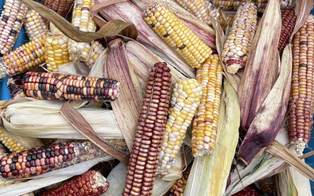
Indigenous Seed Keeping and Seed Climate Adaptation

Challenges, priorities, and multi-sector change in resourcing and advancing Indigenous agricultural and climate sovereignty

• Nicole Davies

Indigenous Climate Action

How can Indigenous Climate Action and other environmental organizations participate in and uphold appropriate engagement and representation of Inuit knowledge and worldview in climate policy?

• Alexa Metallic

Ceremony is for Us, for Mother Earth

Ceremony and the sacred work of decolonizing climate policy in so-called British Columbia

• Elaine Alec
• Jake Rogger
• Chris Derickson
• Lydia Pengilley

Building heat

Hybrid heat in Quebec: Energir and Hydro-Quebec’s collaboration on building heat decarbonization

A proactive approach to the inevitable decarbonization of our energy system.

• Hugo Séguin
• Alex Bigouret

Heat pumps are hot in the Maritimes

The policies and forces driving widespread uptake.

• Chris Turner

St. Laurent North denied

What a decision on an Enbridge gas pipeline in Ottawa tells us about the energy transition.

• Mitchell Beer

Mobilizing private capital to support Canada’s clean growth

Australia’s Green Bank

Canada can draw lessons from Australia’s Green Bank to help the Canada Infrastructure Bank and the Canada Growth Fund define or improve their principles and approach.

• Katherine Monahan
• Marisa Beck

The United Kingdom’s contracts for difference policy for renewable electricity generation

Canada can apply several lessons from the United Kingdom’s Contracts for Difference policy for renewable electricity generation.

Hydrogen tax credits in the U.S. Inflation Reduction Act

What are the U.S. hydrogen tax credits and how their design can inform Canada’s support for hydrogen fuels.

Longship carbon capture and storage in Norway’s North Sea

Longship’s example shows how Canada could optimize its comparative advantages in its climate-related and carbon capture investments.

Clean electricity

Nordic co-operation, Canadian provincialism

Clean power lessons from Nordic efforts to expand electricity trade and decarbonize the grid.

• Shawn McCarthy

Germany’s Energiewende 4.0 Project

Lessons for Canada’s electricity system transformation

Just transition

Managing a just transition in Denmark

With strong market signals, innovation and investment in renewable energy takes the lead.

• Tamara Krawchenko

Managing a just transition in Scotland

A national strategy that includes economic transformation and a just transition for high-emitting industries.

Managing a just transition in New Zealand’s Taranaki Region

A proactive, place-based, and regional partnership approach.

Indigenous perspectives

The power of Acimowin (Storytelling) for climate change policy

Explore the power of story and the medicine wheel as a learning pedagogy and how Indigenous ways of knowing and being should inform adaptation and policy decisions.

• Sandra Lamouche

Hope flows from action: Rebuilding with resilient foundations in B.C.’s Fraser Canyon Region

Policy approaches can help build—and rebuild—communities so they are resilient to the weather of today and tomorrow.

• Patrick Michell

Community is the solution

The 2021 extreme heat emergency experience in urban, rural, and remote British Columbia First Nations.

• Lilia Yumagulova
• Emily Dicken
• Sheri Lysons
• Casey Gabriel
• Randy Carpenter

The Bagida’waad Alliance: Finding our way in the fog and charting a new course

Adapting to the impacts of climate change on the Great Lakes.

• Natasha Akiwenzie
• Victoria Serda
• James Stinson

A Two-Roads Approach to Co-Reclamation: Centring Indigenous voices and leadership in Canada’s energy transition

To adequately prepare for the energy transition, the oil and gas sector must reckon with the historic and ongoing impacts on the land and on Indigenous rights holders.

ʔuyaasiłaƛ n̓aas, or Something happened to the weather

Applying the wisdom of Indigenous place names in a changing climate—lessons from the Ahousaht First Nation’s Land Use Vision process

Gitxsan Rez-ilience

Understanding climate resilience as Naadahahlhakwhlinhl (interconnectedness)

Decolonizing Canada’s Climate Policy

The first step is to decolonize systems that exclude Indigenous rights holders, land protectors, and knowledge experts from the conversation.

• Rebecca Sinclair

Indigenomics: Our Eyes on the Land

Re-valuing Indigenous worldview in today’s climate response

• Carol Anne Hilton

“Our people have borne witness to climate change through deep time”

Indigenous place-based people transitioning to a low-carbon economy

• Frank Brown

Indigenous partnerships—the key to meeting Canada’s climate commitments?

Indigenous clean energy partnerships will play a critical role in the low-carbon transition

• Tabatha Bull

Protecting Biocultural Heritage and Land Rights

How the W8banaki Nation is Adapting to Climate Change in Southern Quebec

• Suzie O’Bomsawin
• Jean-François Provencher
• Samuel-Dufour Pelletier

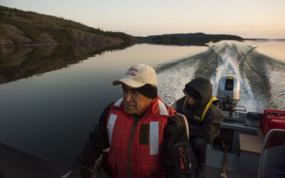
The ‘Two-Eyed Seeing’ of Cross-Cultural Research Camps

Sahtú community-led approaches to climate change monitoring are building the knowledge and capacity needed for adaptation 

• Kirsten Jensen
• Leon Andrew
• Deborah Simmons

Climate Change impacts on bees in Mi’kma’ki

Lessons from the Mi’kmaq Pollinator Project

• Gregory Dugas

Environmental Racism and Climate Change: Determinants of Health in Mi’kmaw and African Nova Scotian Communities

Addressing the structural determinants of health can bring us closer to achieving health equity in Canada and building resilience to climate change.

• Ingrid Waldron

Seed Sowing

Indigenous Relationship-Building as Processes of Environmental Action

• Elisabeth Miltenburg
• Hannah Tait Neufeld
• Laura Peach
• Sarina Perchak

Ayookxw Responding to Climate Change

The Gitanyow are using both Indigenous knowledge and laws (Ayookxw) and western science to build a comprehensive understanding of the ecological health of our territory, and translating that knowledge into policies that respond to the impacts of climate change.

• Tara Marsden
• Deborah Curran

Unnatural Disasters

Colonialism, climate displacement, and Indigenous sovereignty in Siksika Nation’s disaster recovery efforts

• Darlene Yellow Old Woman-Munro

Climate adaptation

Flood Vulnerability and Climate Change

Improving flood risk assessment by mapping socioeconomic vulnerability in a mid-sized Canadian city

• Liton Chakraborty
• Jason Thistlethwaite
• Daniel Henstra

Enhancing Community Resilience as Wildfire Risk Increases

As climate change increases the risk of wildfires, which tools are effective in supporting local action and building capacity in communities?

Resilient cities

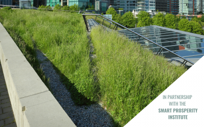
Can Green Roofs Help Cities Respond to Climate Change?

Green roofs help to cool the air, absorb excess water, and reduce energy use while supporting biodiversity and making cities more liveable.

Growing Forests in a City

Forests deliver many benefits to cities, including offering refuge in heatwaves, sequestering greenhouse gas emissions, limiting flooding, and providing mental and physical health benefits.

Wetlands Can Be Infrastructure, Too

Protecting and restoring wetlands will be critical to reducing climate-driven flood risks and slowing biodiversity loss.

Clean growth

Permitting reform for clean energy projects in New York and California

Promising changes at the state level may hold useful lessons for Canada

• Jonathan Arnold

Clean Growth in Nova Scotia

Nova Scotia provides a tangible example of what clean growth means in practice. The province has significantly reduced its greenhouse gas emissions since 2005 while growing its economy.

Climate legislation

Greater than the sum of its parts

How a whole-of-government approach to climate change can improve Canada’s climate performance

• Janetta McKenzie
• Jonas Kuehl

Climate Legislation in British Columbia

This case study explores the core features of B.C.’s amended Climate Change Accountability Act 2019. The legislation mandates the setting of sectoral and interim emissions reduction targets, regular reporting requirements and establishes an independent expert advisory body to provide advice.

Manitoba’s Climate and Green Plan Implementation Act 2018

In 2018, Manitoba became the first province in Canada to implement climate accountability legislation. Its legislation does not include long-term emissions reductions targets or a clearly-defined emissions reduction pathway. Manitoba’s approach and experience offers valuable lessons for Canadian governments contemplating broader climate accountability legislation. 

Climate Legislation in Aotearoa/New Zealand

Aoteroa/New Zealand created climate legislation that enshrines long-term emissions reduction targets. Their legislation is notable for its emphasis on engagement, recognition, and inclusion of iwi and Māori throughout the development and implementation process.

Climate Legislation in the United Kingdom

Reviewing the six defining features of the UK’s 2008 Climate Change Act, the first law to make long-term emissions reduction targets legally binding. What lessons does this legislation have for Canada?

McCombs School of Business

• Español ( Spanish )

Videos Concepts Unwrapped View All 36 short illustrated videos explain behavioral ethics concepts and basic ethics principles. Concepts Unwrapped: Sports Edition View All 10 short videos introduce athletes to behavioral ethics concepts. Ethics Defined (Glossary) View All 58 animated videos - 1 to 2 minutes each - define key ethics terms and concepts. Ethics in Focus View All One-of-a-kind videos highlight the ethical aspects of current and historical subjects. Giving Voice To Values View All Eight short videos present the 7 principles of values-driven leadership from Gentile's Giving Voice to Values. In It To Win View All A documentary and six short videos reveal the behavioral ethics biases in super-lobbyist Jack Abramoff's story. Scandals Illustrated View All 30 videos - one minute each - introduce newsworthy scandals with ethical insights and case studies. Video Series

Case Study UT Star Icon

Climate Change & the Paris Deal

While climate change poses many abstract problems, the actions (or inactions) of today’s populations will have tangible effects on future generations.

In December 2015, representatives from 195 nations gathered in Paris and signed an international agreement to address climate change, which many observers called a breakthrough for several reasons. First, the fact that a deal was struck at all was a major accomplishment, given the failure of previous climate change talks. Second, unlike previous climate change accords that focused exclusively on developed countries, this pact committed both developed and developing countries to reduce greenhouse gas emissions. However, the voluntary targets established by nations in the Paris climate deal fall considerably short of what many scientists deem necessary to achieve the stated goal of the negotiations: limiting the global temperature increase to 2 degrees Celsius. Furthermore, since the established targets are voluntary, they may be lowered or abandoned due to political resistance, short-term economic crises, or simply social fatigue or disinterest.

As philosophy professor Stephen Gardiner aptly explains, the challenge of climate change presents the world with several fundamental ethical dilemmas. It is simultaneously a profoundly global, intergenerational, and philosophical problem. First, from a global perspective, climate change presents the world with a collective action problem: all countries have a collective interest in controlling global carbon emissions. But each individual country also has incentives to over-consume (in this case, to emit as much carbon as necessary) in response to societal demands for economic growth and prosperity.

Second, as an intergenerational problem, the consequences of actions taken by the current generation will have the greatest impact on future generations yet to be born. Thus, the current generation must forego benefits today in order to protect against possibly catastrophic costs in the future. This tradeoff is particularly difficult for developing countries. They must somehow achieve economic growth in the present to break out of a persistent cycle of poverty, while limiting the amount of greenhouse gasses emitted into the atmosphere to protect future generations. The fact that prosperous, developed countries (such as the U.S. and those in Europe) arguably created the current climate problems during their previous industrial economic development in the 19th and 20th centuries complicates the tradeoffs between economic development and preventing further climate change.

Finally, the global and intergenerational nature of climate change points to the underlying philosophical dimensions of the problem. While it is intuitive that the current generation has some ethical responsibility to leave an inhabitable world to future generations, the extent of this obligation is less clear. The same goes for individual countries who have pledged to reduce carbon emissions to help protect environmental health, but then face real economic and social costs when executing those pledges. Developing nations faced with these costs may encounter further challenges as the impact of climate change will most likely fall disproportionally on the poor, thus also raising issues of fairness and inequality.

Discussion Questions

1. On the one hand, what harms are potentially produced by failing to take action to control climate change? On the other hand, what harms are potentially produced by acting to lower carbon emissions?

2. To what extent do humans have a moral responsibility to future generations that are yet to be born? Explain your reasoning.

3. Arguably, actions to cut carbon emissions and curb global warming right now have real costs for certain segments of the global population while the benefits of such actions are more abstract. How should we balance the tangible costs in the present and abstract consequences in the future when addressing climate change? Explain.

4. If you were in a position to recommend environmental policy changes or actions, what would you advocate and why?

5. Do prosperous countries have a greater responsibility to take action and bear more of the costs of controlling climate change than developing countries? Explain your reasoning.

6. Considering that the negative impacts of climate change will likely fall disproportionally on the poor, yet developing countries must often increase consumption and emissions to achieve greater economic growth, do you think developing nations should be exempt from actions to control climate change? Why or why not?

7. The climate change agreement approved in Paris is based on voluntary goals and pledges by participating countries. Would it be ethically permissible to impose carbon emission goals on countries and individuals and enforce them with penalties? Explain your reasoning.

Related Videos

Tangible & Abstract

Tangible and abstract describes how we react more to vivid, immediate inputs than to ones removed in time and space, meaning we can pay insufficient attention to the adverse consequences our actions have on others.

Bibliography

Nations Approve Landmark Climate Accord in Paris http://www.nytimes.com/2015/12/13/world/europe/climate-change-accord-paris.html

Climate Model Predicts West Antarctic Ice Sheet Could Melt Rapidly http://www.nytimes.com/2016/03/31/science/global-warming-antarctica-ice-sheet-sea-level-rise.html

What Does a Climate Deal Mean for the World? http://www.nytimes.com/interactive/2015/12/12/science/What-Does-the-Climate-Deal-Mean.html

Peter Singer on the COP21 Agreement and the Ethics of Climate Change https://www.good.is/articles/peter-singer-climate-cop21-agreement

The Ethical Dimension of Tackling Climate Change http://e360.yale.edu/feature/the_ethical_dimension_of_tackling_climate_change/2456/

Here’s what political science can tell us about the Paris climate deal https://www.washingtonpost.com/news/monkey-cage/wp/2015/12/14/heres-what-political-science-can-tell-us-about-the-paris-climate-deal/

Stay Informed

Support our work.

Browser does not support script.

• LSE Research for the World Strategy
• LSE Expertise: Global politics
• LSE Expertise: UK Economy
• Find an expert
• Research for the World magazine
• Research news
• LSE iQ podcast
• LSE Festival
• Researcher Q&As

Impact case study

An economic solution to climate change that could save trillions.

  Thank you to the Grantham Research Institute of the LSE for their hard work behind the scenes. Christiana Figueres Executive Secretary of the United Nations Framework Convention on Climate Change

Research by

Professor Simon Dietz

Department of geography and environment, prof. sam fankhauser, director, grantham research institute on climate change and the environment.

LSE research helped governments worldwide put a price on carbon that could curb harmful emissions and save $1 trillion annually

What was the issue?

Amid rising concern over the impact of climate change, policymakers have been looking at ways to reduce carbon emissions.

''For economists the problem is that polluters are not required to bear the full cost of the pollution they create in terms of the costs to wider society.''

Economists have argued that putting a “price” on carbon, so that polluters are forced to take into account the negative effects of their harmful emissions, must be a core element of an economically efficient strategy to curb these emissions.

However, the pricing of carbon emissions is by no means an easy or straightforward undertaking. The approaches to such pricing are numerous, complex and competing, making it particularly challenging for policymakers, many with only a layperson's understanding, to decide on an optimal approach.

The stakes are huge. Estimates suggest that the cost savings from an economically efficient policy intervention could be as high $1 trillion a year globally.

What did we do?

Many countries such as the UK use cost-benefit analysis to evaluate new spending and regulations. The original approach used to price a ton of emissions was the so-called “social cost of carbon” - the economic value of the damage caused by an extra ton of greenhouse gases in the atmosphere.

The Stern Review on the Economics of Climate Change (2006) estimated the total cost of climate change to be equivalent to a one-off, permanent 5-20% loss in global average (mean) per-person spending in today’s money. The cost of each extra ton of carbon emitted today was estimated to be around $312.

Researchers at LSE's Grantham Research Institute on Climate Change and the Environment, led by Associate Professor Simon Dietz, subsequently updated the economic modelling that they had produced for the Stern Review.

They showed that the social cost of carbon that had been used in the Stern Review had a high level of uncertainty. They concluded that the most robust measure of the price of carbon for cost-benefit analysis should be the cost of cutting each extra ton of emissions.

Professor Sam Fankhauser and colleagues also looked at the specific tools being proposed to impose a price on carbon, such as carbon taxes and cap-and-trade. The latter was an approach in which governments set a limit or "cap" on certain types of emissions and polluting companies could sell or "trade" the unused portion of their limits to companies that were struggling to comply.

The researchers examined important design elements of cap-and-trade systems. These included: how to bank and borrow emissions permits and how this process interacted with other markets, taxes and subsidies; and ways to keep the permit price from rising too high or falling too low.

They also documented how carbon pricing policies had been implemented across the world so that countries could learn about what other jurisdictions were doing and become aware of good ideas and practices being tested elsewhere.

“Thank you to the Grantham Research Institute of the LSE for their hard work behind the scenes.”

 - Christiana Figueres, Executive Secretary of the United Nations Framework Convention on Climate Change.

What happened?

The research has influenced both the policy thinking as well as the design and substance of carbon pricing legislation in the UK and elsewhere in the world.

Carbon pricing in the UK

In 2009 the UK Department for Energy and Climate Change (DECC) changed its guidance on the price of carbon for cost-benefit analysis, from using the social cost of carbon to using the marginal cost of cutting emissions, as the LSE research had proposed.

DECC's report cited Dietz, who had been one of six independent peer-reviewers of the interim guidance produced in 2007. He was employed as a consultant by DECC for the preparation of the new guidance in 2008/2009.

This change in carbon pricing was expected to increase the likelihood that the UK government would meet its statutory obligation per the Climate Change Act of reducing overall emissions by at least 26% by 2020 and 80% by 2050.

Carbon pricing worldwide

The research has also had an impact on legislation to introduce new carbon pricing policies in Australia, China, Mexico and South Korea, all of which have adopted new measures or are in the process of doing so.

The United Nations has referred to the Grantham research as contributing to the prospects for an international agreement on climate change.

The research was also used as the basis of discussions between UK and EU legislators and China’s chief negotiator, Minister Xie Zhenhua, in the House of Commons in October 2011 when the two sides examined examples of “good practice”.

The researchers have worked closely with GLOBE International, a global forum of parliamentarians. Their research fed directly into an international policy paper that aimed to help national legislators understand the nuts and bolts of carbon markets as they draft their own country-specific legislation.

The LSE team also provided direct advice on a particular technical point of the Australian trading scheme related to the treatment of carbon offsets (credits that can be earned by reducing greenhouse gas emissions in one location that can offset pollution elsewhere).

Search all impact case studies.

Related content

Designing a global agreement on climate change finance, ensuring the best science-based predictions of climate change, using philosophy to improve dutch climate change and sustainability policies, helping the palestinian territory adapt to climate change, more by simon dietz, optimal climate policy under exogenous and endogenous technical change: making sense of the different approaches.

Author(s) Simon Dietz

Optimal climate policy as if the transition matters

Growth and adaptation to climate change in the long run.

What do global climate change and global warming look like? Surface temperature statistics paint a compelling picture of the changing climate: 2023, according to the European Union (link resides outside of ibm.com) climate monitor Copernicus, was the warmest year on record—nearly 1.5 degrees Celsius warmer than pre-industrial levels.

To gain a holistic understanding of the current climate crisis and future climate implications, however, it’s important to look beyond global average temperature records. The impacts of climate change may be organized into three categories:

• Intensifying extreme weather events
• Changes to natural ecosystems
• Harm to human health and well-being

While climate change is defined as a shift in long-term weather patterns, its impacts include an increase in the severity of short-term weather events.

• Heat waves: Dangerous heat waves are becoming more common and are one of the most obvious effects of climate change as the Earth’s temperature continues to rise.
• Droughts: Higher temperatures can cause faster water evaporation, making arid regions even more dry. Climate change-linked shifts in atmospheric circulation can further exacerbate drought conditions as rain bypasses dry regions.
• Wildfires: Droughts and faster water evaporation can lead to drier vegetation, fueling larger and more frequent wildfires. According to NASA (link resides outside of ibm.com), even typically rainy regions will be more vulnerable to wildfires and wildfire seasons are extending around the globe.
• Heavy rain and tropical storms: Climate change alters precipitation patterns, with NASA reporting more frequent periods of excess precipitation. Scientists project further increases (link resides outside of ibm.com) in tropical cyclone rainfall in particular, due to greater atmospheric moisture content.
• Increased coastal flooding: Sea level rises associated with global warming are leaving low-lying coastal areas vulnerable to greater flooding, according to the Intergovernmental Panel on Climate Change (IPCC, link resides outside of ibm.com).

Due to climate change, natural ecosystems are undergoing long-term changes and declines in biodiversity. Here are a few examples:

• Sea ice loss and melting ice sheets: Declining levels of Arctic sea ice threaten the habitats of species such as polar bears and walruses. Polar bears hunt seals in the Arctic sea ice habitat while walruses rely on the ice as a place to rest when they’re not diving for food. In Greenland and Antarctica, melting ice sheets are contributing to rising sea levels, endangering coastal ecosystems around the world.
• Damage to coral reefs: Ocean temperature increases in warmer climates from Australia to Florida are causing coral reefs to lose colorful algae, leading to what’s known as “coral bleaching.”
• Ocean acidification: Marine life is also at risk from ocean acidification, stemming from greenhouse gas emissions and the greater concentration of carbon dioxide in the atmosphere. That carbon dioxide is absorbed by seawater, leading to chemical reactions that make oceans more acidic. Shellfish are especially vulnerable to ocean acidification, which NOAA describes as having “osteoporosis-like effects” on oysters and clams.
• Invasive species proliferation: Warmer temperatures allow invasive species to move to new areas, often to the detriment of native wildlife. The spread of the purple loosestrife plant in North America, for instance, has reduced nesting sites and resulted in the decline of some bird populations.
• Harm to estuarine ecosystems: Droughts reduce freshwater flows and increase salinity in estuaries, while greater precipitation increases stormwater runoff, introducing more sediment and pollution. These changes threaten the wildlife that rely on specific estuarine conditions to thrive.

Climate change is increasingly impacting the quality of life on Earth, affecting people’s health and economic well-being.

• Illnesses and fatalities: Rising global temperatures foster conditions for infectious diseases to spread, and extreme weather events cause tragic loss of life as well as illnesses. Poor air quality from wildfire smoke can exacerbate asthma and heart disease, for example, while heat waves can cause heat exhaustion. More than 60,000 people (link resides outside of ibm.com) died in European heat waves in 2022.
• Food insecurity: Droughts and scarcity of water supplies, severe storms, extreme heat and invasive species can cause crop failures and food insecurity. Most of those at risk of climate change-linked hunger are in Sub-Saharan Africa, South Asia and Southeast Asia, according to the World Bank (link resides outside of ibm.com).
• Financial consequences: Climate change can hurt businesses and individuals’ financial well-being. For example, changing weather patterns have imperiled wine production in California, while rising sea levels threaten the future of Caribbean coastal resorts. Meanwhile, insurance companies are increasingly declining to provide property insurance in areas vulnerable to extreme weather, leaving homeowners there at greater financial risk.
• Damage to infrastructure: Wildfires, powerful storms and flooding can damage energy grids , leading to power outages, as well as transportation networks, hindering people’s ability to access services and goods to meet their daily needs. Damage to one type of infrastructure can lead to consequences for another: As noted by the U.S. government’s National Climate Assessment  (link resides outside of ibm.com), “failure of the electrical grid can affect everything from water treatment to public health.”

Though some of the impacts on Earth’s climate are irreversible, a wide range of organizations from the public and private sector are working on climate actions that address the causes of climate change. These include ongoing mitigation strategies and targets for the reduction of greenhouse gas emissions, such as emissions of carbon dioxide and methane.

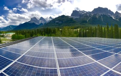
Meeting these targets relies in part on the growth of clean, renewable energy production that reduces the world’s reliance on energy derived from the burning of fossil fuels. Other climate science innovation could also contribute to climate change mitigation measures, ranging from carbon capture technology to methods of neutralizing ocean acidity (link resides outside of ibm.com).

Existing sustainable technologies can also help companies lower their carbon footprint. Artificial intelligence-powered analysis, for example, can help companies identify what parts of their operations produce the most greenhouse gas emissions; carbon accounting can inform their strategies on reducing those emissions.

Of utmost importance, scientists say, is acting quickly.

“If we act now,” IPCC Chair Hoesung Lee said in a 2023 statement (link resides outside of ibm.com), “we can still secure a livable sustainable future for all.”

Put your sustainability initiatives into action by managing the economic impact of severe weather and climate change on your business practices through the IBM Environmental Intelligence Suite .

Explore sustainability strategy

Learn about climate and weather risk management

An enquiry into rehabilitation as a climate change adaptation policy: the case of the Western Ghats of Kerala, India

• Published: 29 August 2024
• Volume 89 , article number  201 , ( 2024 )

Cite this article

• Renjith Raj   ORCID: orcid.org/0000-0001-5090-6220 1 &
• Arfat Ahmad Sofi 2  

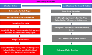
The Western Ghats have been declared as a World Heritage Site by UNESCO. Besides, it is classified as one of the world’s 36 biodiversity hotspots by Conservation International. The Western Ghats of Kerala have experienced devastating landslides and floods in recent years, which are triggered by climate change. This alarming situation calls for policymakers to develop a comprehensive climate adaptation policy at the local level. However, no study has yet thoroughly investigated this critical issue. Therefore, this study explores the prospects and trade-offs of climate rehabilitation policies for families living in the highly landslide- and flood-prone areas of the Western Ghats in Kerala, India. We have undertaken a mixed methodology comprising four focus group discussions followed by empirical analyses. Towards this, a semi-structured questionnaire is framed to gather relevant information based on the outcomes. The data are analyzed using robust logistic regression models. The findings indicate that most agricultural worker families support the rehabilitation policy, given their lower opportunity costs due to the absence of farmland ownership. On the other hand, agricultural families face considerable trade-offs regarding rehabilitation. Most agricultural families prefer to rehabilitate within a short distance from the current residence or construct a retaining wall as they fear rehabilitation to distant places will gravely affect their livelihood. This research highlights the potential for implementing a rehabilitation policy for marginalized communities heavily exposed to climate risks. Additionally, constructing retaining walls should also be a primary focus of the Government.

This is a preview of subscription content, log in via an institution to check access.

Access this article

Subscribe and save.

• Get 10 units per month
• Download Article/Chapter or eBook
• 1 Unit = 1 Article or 1 Chapter
• Cancel anytime

Price includes VAT (Russian Federation)

Instant access to the full article PDF.

Rent this article via DeepDyve

Institutional subscriptions

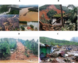
Source: The Indian Express.Note: "Panel A: Aerial images of the Kerala floods, August 2018. Panel B: Kavalappara, Malappuram district, landslides occurred on August 8, 2019, which led to a casualty of 59 people. Panel C: Pettimudi, Idukki district, landslides occurred on August 7, 2020, where 70 people were buried alive. Panel D: Kootickal village bordering Idukki and Kottayam districts, landslides occurred on October 17, 2021, which led to a death toll of 15"

Source : Report of the Western Ghats Ecologically Expert Panel (2011)

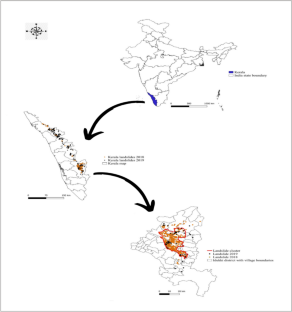
Source: Kerala State Disaster Management Authority

The state of Kerala lies in the southern part of the west coast of India.

Mesoscale cloudburst is the technical term to indicate a rainfall of 50 mm in 2 h.

Rainfall erosivity is an index that describes the power of rainfall to cause soil erosion.

Achu, A. L., Thomas, J., Aju, C. D., Vijith, H., & Gopinath, G. (2024). Redefining landslide susceptibility under extreme rainfall events using deep learning. Geomorphology, 448 , 109033.

Article   Google Scholar  

Assam state disaster management authority. 2022. In Assam flood report 2022.

Bahinipati, C. S., & Patnaik, U. (2020). Does development reduce damage risk from climate extremes? Empirical evidence for floods in India. Water Policy, 22 (5), 748–767. https://doi.org/10.2166/wp.2020.059

Barua, P., Rahman, S. H., & Molla, M. H. (2017). Sustainable adaptation for resolving climate displacement issues of south eastern islands in Bangladesh. International Journal of Climate Change Strategies and Management., 9 (6), 790–810. https://doi.org/10.1108/IJCCSM-02-2017-0026

Eckstein, D,. Kunzel, V., Schafer, L., Winges, M., (2020). GLOBAL CLIMATE RISK INDEX 2020. In Who suffers most from extreme weather events? Weather – related loss events in 2018 and 1999 to 2018. GERMANWATCH. Briefing paper.

Gadgil M., (2011). Report of the western ghats ecologically expert panel. In Ministry of environment, forests and climate change, government of India.

Gopinath, G., Jesiya, N., Achu, A, L., Bhadran, A., Surendran, U, P., (2023). Ensemble of fuzzy-analytical hierarchy process in landslide susceptibility modeling from a humid tropical region of Western Ghats, Southern India. In Environmental science and pollution research.

Gorman, C. E., Torsney, A., Gaughran, A., McKeon, C. M., Farrell, C. A., White, C., Donohue, I., Stout, J. C., Buckley, Y. M., (2023). Reconciling climate action with the need for biodiversity protection, restoration and rehabilitation. In Science of the total environment. 857, Part 1.

Government of Kerala. (2020). Memorandum: Kerala Floods – 2019.

Gupta, V., & Jain, M. K. (2020). Impact of ENSO, global warming, and land surface elevation on extreme precipitation in India. Journal of Hydrologic Engineering., 25 , 1.

Haque, U., da Silva, P. F., Devoli, G., Pilz, J., Zhao, B., Khaloua, A., Wilopo, W., Andersen, P., Lu, P., Lee, J., Yamamoto, T., Keelings, D., Wu, J. H., & Glass, G. E. (2019). The human cost of global warming: deadly landslides and their triggers (1995–2014). Science of the Total Environment., 682 , 673–684. https://doi.org/10.1016/j.scitotenv.2019.03.415

Hunt, K. M. R., & Menon, A. (2020). The 2018 Kerala floods: a climate change perspective. Climate Dynamics., 54 (3–4), 2433–2446.

IPCC. (2022). Climate change 2022: impacts, adaptation and vulnerability. In summary for policymakers.

IPCC. (2023). Assessment round 6 synthesis report: climate change 2023.

Irshad, S. M., & Solaman, S. S. C. (2022). Identity, space and disaster: a case study of Pettimudi landslide in Kerala. In Sociological Bulletin., 71 (3), 437–453. https://doi.org/10.1177/00380229221094785

Kerala Forest Department., (2021). Kerala forests statistics 2021. In Government of Kerala.

Krishnan, R., Sanjay, J., Gnanaseelan, Chellappan., Mujumdar, Milind., Kulkarni, Ashwini., Chakraborty, Supriyo., (2020). Assessment of climate change over the Indian region. In A report of the ministry of earth science (MoES), government of India.

Kumar, P., & Brewster, C. (2022). Co-production of climate change vulnerability assessment-a case study of the Indian lesser Himalayan region. Darjeeling. Journal of Integrative Environmental Sciences., 19 (1), 39–64. https://doi.org/10.1080/1943815X.2022.2033792

Kumar, P. V., & Naidu, C. V. (2020). Is pre-monsoon rainfall activity over india increasing in the recent era of global warming? Pure and Applied Geophysics., 177 , 4423–4442. https://doi.org/10.1007/s00024-020-02471-7

Li, B. V., Jenkins, C, N., Xu, W., (2022). Strategic protection of landslide vulnerable mountains for biodiversity conservation under land-cover and climate change impacts. In Proceedings of the national academy of sciences united states of America. 119(2).

Mishra, Anoop, & Kumar., Nagaraju, V., Rafiq, Mohammd., Chandra, Sagarika. (2018). Evidence of links between regional climate change and precipitation extremes over India. Royal Meteorological Society., 74 (6), 218–221. https://doi.org/10.1002/wea.3259

Mittermeier, R. A., Myers, N., Mittermeier, C. G., Robles, G, P., (1999). Hotspots: earth’s biologically richest and most endangered terrestrial ecoregions. In Conservation international.

Oeba, V. O., & Larwanou, M. (2017). Forestry and resilience to climate change: a synthesis on application of forest-based adaptation strategies to reduce vulnerability among communities in sub-Saharan Africa (pp. 153–168). Cham: Climate Change Adaptation in Africa Springer.

Google Scholar  

Oomen, V. O., (2014). Understanding report of the western ghats ecologically expert panel, Kerala perspective. In Kerala state biodiversity board.

Panagos, Panos, Borrelli, Pasquale, Matthews, Francis, Liakos, Leonidas, Bezak, Nejc, Diodato, Nazzareno, & Ballabio, Cristiano. (2022). Global rainfall erosivity projections for 2050 and 2070. Journal of Hydrology, 610

Paramesh, V., Kumar, P., Shamim, M., Ravisankar, N., Arunachalam, V., Nath, A. J., Mayekar, T., Singh, R., Prusty, A. K., Rajkumar, R. S., Panwar, A. S., Reddy, V. K., Pramanik, M., Das, A., Manohara, K. K., Babu, S., & Kashyap, P. (2022). Integrated farming systems as an adaptation strategy to climate change: case studies from diverse agro-climatic zones of India. Sustainability, 14 (18), 11629. https://doi.org/10.3390/su141811629

Pramanik, M., Chowdhury, K., Rana, M. J., Bisht, P., Pal, R., Szabo, S., Pal, I., Behera, B., Liang, Q., Padmadas, S. S., & Udmale, P. (2022a). Climatic influence on the magnitude of COVID-19 outbreak: A stochastic model-based global analysis. International Journal of Environmental Health Research, 32 (5), 1095–1110. https://doi.org/10.1080/09603123.2020.1831446

Pramanik, M., Diwakar, A. K., Dash, P., Szabo, S., & Pal, I. (2021a). Conservation planning of cash crops species (Garcinia gummi-gutta) under current and future climate in the Western Ghats, India. Environment, Development and Sustainability, 23 (4), 5345–5370. https://doi.org/10.1007/s10668-020-00819-6

Pramanik, M., Paudel, U., Mondal, B., Chakraborti, S., & Deb, P. (2018). Predicting climate change impacts on the distribution of the threatened Garcinia indica in the Western Ghats, India. Climate Risk Management, 19 , 94–105. https://doi.org/10.1016/j.crm.2017.11.002

Pramanik, M., Szabo, S., Pal, I., Udmale, P., O’Connor, J., Sanyal, M., Roy, S., & Sebesvari, Z. (2021). Twin disasters: tracking COVID-19 and cyclone Amphan’s impacts on SDGs in the Indian Sundarbans. Environment: science and policy for sustainable development, 63 (4), 20–30. https://doi.org/10.1080/00139157.2021.1924575

Pramanik, M., Szabo, S., Pal, I., Udmale, P., Pongsiri, M., & Chilton, S. (2022b). Population health risks in multi-hazard environments: action needed in the cyclone amphan and COVID-19–hit sundarbans region. India. Climate and Development, 14 (2), 99–104.

Qasim, M., Khan, M., & Rashid, W. (2023). Spatial and temporal analyses of land use changes with special focus on seasonal variation in snow cover in district Chitral; a Hindu Kush mountain region of Pakistan. Remote Sensing Applications: Society and Environment., 29 , 100902. https://doi.org/10.1016/j.rsase.2022.100902

Raj, R., & Sofi, A. A. (2023). Does climate change leads to severe household-level vulnerability? Evidence from the Western Ghats of Kerala. India. Land Use Policy, 130 , 106655.

Reddy, K. V., Paramesh, V., Arunachalam, V., Das, B., Ramasundaram, P., Pramanik, M., Sridhara, S., Reddy, D. D., Alataway, A., Dewidar, A. Z., & Mattar, M. A. (2022). Farmers’ perception and efficacy of adaptation decisions to climate change. Agronomy, 12 (5), 1023. https://doi.org/10.3390/agronomy12051023

Roxy, M. K., Ghosh, S., Pathak, A., Athulya, R., Mujumdar, M., Murtugudde, R., Terray, P., & Rajeevan, M. (2017). A threefold rise in widespread extreme rain events over central India. Nature Communications., 8 (1), 708. https://doi.org/10.1038/s41467-017-00744-9

Samui, S., & Sethi, N. (2022). Social vulnerability assessment of glacial lake outburst flood in a northeastern state in India. International Journal of Disaster Risk Reduction., 74 , 102907. https://doi.org/10.1016/j.ijdrr.2022.102907

Sharma, J., Upgupta, S., Kumar, R., Chaturvedi, R. K., Bala, G., & Ravindranath, N. H. (2015). Assessment of inherent vulnerability of forests at landscape level: a case study from western ghats in India. Mitigation and Adaptation Strategies for Global Change., 22 (1), 29–44.

Sreenath, A. V., Abhilash, S., Vijayakumar, P., & Mapes, B. E. (2022). West coast India’s rainfall is becoming more convective. npj Climate and Atmospheric Science . https://doi.org/10.1038/s41612-022-00258-2

Sultana, N., & Tan, S. (2021). Landslide mitigation strategies in southeast Bangladesh: lessons learned from the institutional responses. International Journal of Disaster Risk Reduction., 62 , 102402. https://doi.org/10.1016/j.ijdrr.2021.102402

Tiwari, P., & Shukla, J. (2022). Post-disaster reconstruction, well-being and sustainable development goals: a conceptual framework. Environment and Urbanization Asia., 13 (2), 323–332. https://doi.org/10.1177/09754253221130405

Upadhyaya, A., & RaiKumar, A. K. P. (2022). Anomalous rainfall trends in the north-western Indian Himalayan region (NW-IHR). Theoretical and Applied Climatology., 151 (1–2), 253–272.

Vijaykumar, P., Abhilash, S., Sreenath, A. V., Athira, U. N., Mohanakumar, K., Mapes, B. E., Chakrapani, B., Sahai, A. K., Niyas, T. N., & Sreejith, O. P. (2021). Kerala floods in consecutive years - its association with mesoscale cloudburst and structural changes in monsoon clouds over the west coast of India. Weather and Climate Extremes., 33 , 100339. https://doi.org/10.1016/j.wace.2021.100339

Wang, Y., Xie, X., Shi, J., Zhu, B., Jiang, F., Chen, Y., & Liu, Y. (2022). Accelerated hydrological cycle on the Tibetan Plateau evidenced by ensemble modelling of long-term water budgets. Journal of Hydrology., 615 , 128710. https://doi.org/10.1016/j.jhydrol.2022.128710

Yaduvanshi, A., Nkemelang, T., Bendapudi, R., & New, M. (2021). Temperature and rainfall extremes change under current and future global warming levels across Indian climate zones. Weather and Climate Extremes., 31 (2021), 100291.

Younus, M. A. F. (2016). Adapting to climate change in the coastal regions of Bangladesh: proposal for the formation of community-based adaptation committees. Environmental Hazards., 16 (1), 21–49. https://doi.org/10.1080/17477891.2016.1211984

Download references

Acknowledgements

The authors would like to express their gratitude to the following persons for their wholehearted cooperation and suggestions, without which this study would not have been realized: Sheeba George IAS—Idukki District Collector, Dr. Sekhar Lukose Kuriakose—Member Secretary, Kerala State Disaster Management Authority, Pradeep G.S—Hazard and Risk Analyst, Kerala State Disaster Management Authority, Rajeev T.R—Hazard and Risk Analyst, Idukki District, Government officials of Idukki taluk revenue office, Government officials and representatives of concerned village panchayats, and the residents of the concerned villages.

This work is part of the Ph.D. No funds have been received for this study.

Author information

Authors and affiliations.

Department of Economics, School of Humanities and Social Sciences, JAIN (Deemed-to-be University), Bengaluru, India

Renjith Raj

Department of Economics and Finance, Birla Institute of Technology and Science, Pilani, KK Birla Goa Campus, Sancoale, India

Arfat Ahmad Sofi

You can also search for this author in PubMed   Google Scholar

Corresponding author

Correspondence to Renjith Raj .

Ethics declarations

Conflict of interest.

The authors do not have any conflict of interest to disclose.

Additional information

Publisher's note.

Springer Nature remains neutral with regard to jurisdictional claims in published maps and institutional affiliations.

Landslide Prone Regions in Kerala Source: Achu et al., 2024

Rights and permissions

Springer Nature or its licensor (e.g. a society or other partner) holds exclusive rights to this article under a publishing agreement with the author(s) or other rightsholder(s); author self-archiving of the accepted manuscript version of this article is solely governed by the terms of such publishing agreement and applicable law.

Reprints and permissions

About this article

Raj, R., Sofi, A.A. An enquiry into rehabilitation as a climate change adaptation policy: the case of the Western Ghats of Kerala, India. GeoJournal 89 , 201 (2024). https://doi.org/10.1007/s10708-024-11198-0

Download citation

Accepted : 15 August 2024

Published : 29 August 2024

DOI : https://doi.org/10.1007/s10708-024-11198-0

Share this article

Anyone you share the following link with will be able to read this content:

Sorry, a shareable link is not currently available for this article.

Provided by the Springer Nature SharedIt content-sharing initiative

• Climate change
• Climatic hazards
• Rehabilitation policy
• The western ghats
• Find a journal
• Publish with us
• Track your research

• Election 2024
• Entertainment
• Newsletters
• Photography
• AP Buyline Personal Finance
• AP Buyline Shopping
• Press Releases
• Israel-Hamas War
• Russia-Ukraine War
• Global elections
• Asia Pacific
• Latin America
• Middle East
• Election results
• Google trends
• AP & Elections
• U.S. Open Tennis
• Paralympic Games
• College football
• Auto Racing
• Movie reviews
• Book reviews
• Financial Markets
• Business Highlights
• Financial wellness
• Artificial Intelligence
• Social Media

What has worked to fight climate change? Policies where someone pays for polluting, study finds

FILE - Vehicles move along Interstate 76 ahead of the Thanksgiving Day holiday in Philadelphia, Nov. 22, 2023. (AP Photo/Matt Rourke, File)

FILE - An offshore wind farm is visible from the beach in Hartlepool, England, Nov. 12, 2019. (AP Photo/Frank Augstein, File)

• Copy Link copied

WASHINGTON (AP) — To figure out what really works when nations try to fight climate change, researchers looked at 1,500 ways countries have tried to curb heat-trapping gases. Their answer: Not many have done the job. And success often means someone has to pay a price, whether at the pump or elsewhere.

In only 63 cases since 1998, did researchers find policies that resulted in significant cuts of carbon pollution, a new study in Thursday’s journal Science found.

Moves toward phasing out fossil fuel use and gas-powered engines, for example, haven’t worked by themselves, but they are more successful when combined with some kind of energy tax or additional cost system, study authors concluded in an exhaustive analysis of global emissions, climate policies and laws.

“The key ingredient if you want to reduce emissions is that you have pricing in the policy mix,” said study co-author Nicolas Koch, a climate economist at the Potsdam Institute for Climate Impact Research in Germany. “If subsidies and regulations come alone or in a mix with each other, you won’t see major emission reductions. But when price instruments come in the mix like a carbon energy tax then they will deliver those substantial emissions reductions.”

The study also found that what works in rich nations doesn’t always work as well in developing ones.

Still, it shows the power of the purse when fighting climate change, something economists always suspected, said several outside policy experts, climate scientists and economists who praised the study.

“We won’t crack the climate problem in wealthier nations until the polluter pays,” said Rob Jackson, a Stanford University climate scientist and author of the book Clear Blue Sky. “Other policies help, but nibble around the edges.”

“Carbon pricing puts the onus on the owners and products causing the climate crisis,” Jackson said in an email.

A great example of what works is in the electricity sector in the United Kingdom, Koch said. That country instituted a mix of 11 different policies starting in 2012, including a phaseout of coal and a pricing scheme involving emission trading, which he said nearly halved emissions — “a huge effect.”

Of the 63 success stories, the biggest reduction was seen in South Africa’s building sector, where a combination of regulation, subsidies and labeling of appliances cut emissions nearly 54%.

The only success story in the United States was in transportation. Emissions dropped 8% from 2005 to 2011 thanks to a mix of fuel standards — which amount to regulation — and subsidies.

Yet even the policy tools that seem to work still barely put a dent in ever-rising carbon dioxide emissions. Overall, the 63 successful instances of climate policies trimmed 600 million to 1.8 billion metric tons of the heat-trapping gas, the study found. Last year the world spewed 36.8 billion metric tons of carbon dioxide while burning fossil fuels and making cement.

If every major country somehow learned the lesson of this analysis and enacted the policies that work best, it would only shrink the United Nations “emissions gap” of 23 billion metric tons of all greenhouse gases by about 26%, the study found. The gap is the difference between how much carbon the world is on track to put in the air in 2030 and the amount that would keep warming at or below internationally agreed upon levels.

“It basically shows we have to do a better job,” said Koch, who is also head of the policy evaluation lab at the Mercator Research Institute in Berlin.

Niklas Hohne at Germany’s New Climate Institute, who wasn’t part of the study said: “The world really needs to make a step change, move into emergency mode and make the impossible possible.”

Koch and his team looked at emissions and efforts to reduce them in 41 countries between 1998 and 2022 —so it doesn’t include the United States’ nearly $400 billion in climate-fighting spending package passed two years ago as a cornerstone of President Joe Biden’s environmental policy — and logged 1,500 different policy actions. They bunched the policies in four broad categories — pricing, regulations, subsidies and information — and analyzed four distinct sectors of the economy: electricity, transportation, buildings and industry.

In what Koch called “the reverse causal approach,” the team looked for emission drops of 5% or more in different sectors of countries’ economies and then figured out what caused them with help of observations and machine learning. Researchers compared emissions to similar nations as control groups and accounted for weather and other factors, Koch said.

The team created a statistically transparent approach that others can use to update or reproduce it, including an interactive website where users can choose nations and economic sectors to see what’s worked. And it could eventually be applied to the 2022 Biden climate package, he said. That package was heavy on subsidies.

John Sterman, a management professor at MIT Sloan Sustainability Institute who wasn’t part of the research, said politicians find it easier to pass policies that subsidize and promote low-carbon technologies. He said that’s not enough.

“It’s also necessary to discourage fossil fuels by pricing them closer to their full costs, including the costs of the climate damage they cause,” he said.

Follow Seth Borenstein on X at @borenbears

Read more of AP’s climate coverage at http://www.apnews.com/climate-and-environment

The Associated Press’ climate and environmental coverage receives financial support from multiple private foundations. AP is solely responsible for all content. Find AP’s standards for working with philanthropies, a list of supporters and funded coverage areas at AP.org .

Climate Crisis Survey Reveals Scientists’ Willingness to Act – and Barriers to Action

• Triveni Sheshadri - [email protected]

Media contact:

• Inga Kiderra - [email protected]

Published Date

Topics covered:.

• Climate change

Share This:

Article content.

Increasing global temperatures. Rising sea levels. Shrinking ice sheets. Warmer ocean water. Over the last several decades, scientists worldwide have amassed compelling evidence on climate change. However, little is known about the personal beliefs and attitudes of climate scientists and scientists and academics in other disciplines about what they are or are not doing beyond research to deal with what appears to be accelerated global heating and its impacts on the biosphere.

A large-scale survey conducted by a team of international researchers led by investigators at the University of Amsterdam has found that scientists worldwide and across disciplines are extremely concerned about climate change and its cascading effects on every sphere of life. Many scientists surveyed in the study report making changes in their own lifestyles and engaging in advocacy and protest, and more are willing to do so in the future. Importantly, they also pointed to key psychological, social and institutional barriers to more advocacy and protest.

Adam Aron, professor of psychology in the School of Social Sciences at the University of California San Diego, is a co-author of the study published Aug. 5 in the journal Nature Climate Change .

“Climate change is one of the biggest threats to humanity,” said Aron whose research is now focused on the social psychology of collective action on the climate and ecological crisis. “Governments, corporations and many institutions continue to make empty promises that downplay the level of transformation that’s required to prevent climate breakdown and to equitably adapt societies to deal with the impacts that are already here.”

The researchers surveyed more than 9,000 scientists from 115 countries about their views on climate change and the extent to which they are engaged in climate action. Climate change worried the majority of respondents (83%). Many more (91%) believed that fundamental changes in social, political and economic systems are needed to mitigate the effects of climate change. When asked about their own actions to combat the climate crisis, many said they have already made significant changes to their lifestyle. They were driving less (69%), flying less (51%) and switching to a more plant-based diet (39%).

{/exp:typographee}

Barriers to engagement and action

The researchers found that the majority of scientists who responded to the survey believed in the effectiveness of climate activist groups to bring about positive change. They were also in support of more engagement on the part of the scientific community in climate advocacy and even protest. Their own responses to the crisis included climate advocacy (29%), participation in legal protest (23%) and/or acts of civil disobedience (10%). About half said they would be willing to engage in some of these in the future.

Based on these results, the authors of the study propose a two-step model of engagement. First, in order for scientists to be willing to engage, they need to break through intellectual barriers that impede climate action such as lack of belief in the effectiveness of the actions, lack of identification with activists, lack of knowledge, fear of losing credibility, and fear of repercussions. Second, they need to overcome mostly practical barriers including perceived lack of skills, lack of time, lack of opportunities, and not knowing any groups involved in climate action.

“This study makes clear that scientists from all disciplines are very worried and are calling for fundamental transformation,” Aron said.  “I hope this helps wake people up and that they get engaged, as more and more scientists are.”

About the survey

Out of the 250,000 targeted emails sent to solicit participation in the study, the research team received more than 9,000 survey responses from scientists and academics in 115 countries in various disciplines and career stages. The researchers acknowledge that respondents who were already involved in climate change may have been more likely to self-select to participate in the survey, which could affect the extent to which the reported results reflect the views of the scientific community as a whole.

Learn more about research and education at UC San Diego in: Climate Change

You May Also Like

At the ready: a day in the life of a trauma surgeon, opentopography receives $4 million to support ai-ready access to topographic data for research and education, borderzone breakthrough: a new source of cardiac inflammation, uc san diego’s mandeville art gallery receives grant from new york-based teiger foundation, stay in the know.

Keep up with all the latest from UC San Diego. Subscribe to the newsletter today.

You have been successfully subscribed to the UC San Diego Today Newsletter.

Campus & Community

Arts & culture, visual storytelling.

• Media Resources & Contacts

Signup to get the latest UC San Diego newsletters delivered to your inbox.

Award-winning publication highlighting the distinction, prestige and global impact of UC San Diego.

Popular Searches: Covid-19   Ukraine   Campus & Community   Arts & Culture   Voices

Thwaites Glacier won’t collapse like dominoes as feared, study finds, but that doesn’t mean the ‘Doomsday Glacier’ is stable

Professor of Earth Sciences, Dartmouth College

Disclosure statement

Mathieu Morlighem receives funding from NASA, the National Science Foundation, the Heising Simons Foundation, and Dartmouth College.

View all partners

Antarctica’s Thwaites Glacier got its nickname the “ Doomsday Glacier ” for its potential to flood coastlines around the world if it collapsed. It is already contributing about 4% of annual sea-level rise as it loses ice, and one theory suggests the glacier could soon begin to collapse into the ocean like a row of dominoes.

But is that kind of rapid collapse really as likely as feared? A new study of Thwaites Glacier’s susceptibility to what’s known as marine ice cliff instability offers some hope. But the findings don’t mean Thwaites is stable.

Polar scientist Mathieu Morlighem , who led the study, explains the results.

Why is the Thwaites Glacier so important?

Thwaites Glacier drains a huge area of Antarctica’s ice sheet – about 74,000 square miles (192,000 square kilometers), an expanse bigger than Florida. If a snowflake falls within that drainage system, it will eventually end up as part of an iceberg in the ocean off Thwaites.

What we are seeing with Thwaites Glacier right now is a disaster in slow motion.

The bedrock under Thwaites Glacier sits below sea level and slopes downward going inland , so the glacier gets deeper toward the interior of the ice sheet. Once the glacier begins losing more ice than it gains from new snowfall and starts to retreat, it’s very hard to slow it down because of this slope. And Thwaites is already retreating at an accelerating rate as the climate warms.

Thwaites Glacier holds enough ice to raise global sea level by more than 2 feet (0.65 meters). Once Thwaites starts to destabilize, it also will destabilize neighboring glaciers . So, what happens to Thwaites affects all of the West Antarctic Ice Sheet, and that affects sea-level rise along coastlines everywhere.

What is marine ice cliff instability?

Marine ice cliff instability is a relatively new concept proposed by scientists in the past decade.

Many of the glaciers around Antarctica have huge floating extensions called ice shelves that buttress the glacier and slow its ice flow into the ocean. With the climate warming, we have seen some of these floating extensions collapse, sometimes very rapidly , in the span of a few weeks or months.

If Thwaites’ ice shelf were to collapse, it would expose a very tall ice cliff facing the ocean along its 75-mile (120-kilometer) front . There is only so much force that ice can sustain, so if the cliff is too tall, it will collapse into the ocean.

Once that happens, a new ice cliff farther back would be exposed, and the new cliff would be even taller because it is farther inland. The theory of marine ice cliff instability suggests that if the cliffs collapse quickly enough, that could have a domino effect of ever-higher ice cliffs collapsing one after the other.

However, no one has observed marine ice cliff instability in action. We don’t know if it will happen, because a lot depends on how quickly the ice collapses.

What did you discover about the risk to Thwaites?

When the theory of marine ice cliff instability was first introduced, it used a rough approximation of how ice cliffs might collapse once the ice shelf was gone.

Studies since then have determined that ice cliffs won’t fail systematically until the ice is about 442 feet (135 meters) high. Even at that point, they would fail more slowly than projected until they became much taller.

We used three high-resolution models to explore what this new physical understanding of ice cliff instability would mean for Thwaites Glacier this century.

Our results show that if Thwaites’ entire ice shelf collapsed today, its ice front would not rapidly retreat inland due to marine ice cliff instability alone. Without the ice shelf, the glacier’s ice would flow much faster toward the ocean, thinning the front of the glacier. As a result, the ice cliffs wouldn’t be as high.

We found that Thwaites would remain fairly stable at least through 2100. We also simulated an ice shelf collapse in 50 years, when the glacier’s grounding line – where its grounded ice meets the ocean – would have retreated deeper inland. Even then, we found that marine ice cliff instability alone would not cause a rapid retreat.

The results call into question some recent estimates of just how fast Thwaites might collapse. That includes a worst-case scenario that the Intergovernmental Panel on Climate Change mentioned in its latest assessment report but labeled as “low likelihood.”

Thwaites is the glacier everyone is worried about. If you model the entire ice sheet, this is where marine ice cliff instability starts and where it propagates far inland . So, if Thwaites isn’t as vulnerable to ice cliff failure as we thought, that’s a good sign for the entire ice sheet.

But marine ice cliff instability is only one mechanism of ice loss. This finding doesn’t mean Thwaites is stable.

What else is causing glaciers to retreat at an accelerating rate?

There are many processes that make the Antarctic ice sheet unstable, some of them very well understood.

Ice-ocean interactions explain most of the recent ice mass loss so far. Antarctica is a very cold place , so atmospheric warming isn’t having a large effect yet. But warm ocean currents are getting under the ice shelves, and they are thinning the ice from below , which weakens the ice shelves. When that happens, the ice streams flow faster because there is less resistance.

Over the past few decades , the Amundsen Sea sector, where Thwaites and Pine Island glaciers are located, has seen an intrusion of warm water from the Antarctic Circumpolar Current, which has been melting the ice from below .

What does climate change have to do with it?

Antarctica can seem like a faraway place, but human activities that warm the planet – such as burning fossil fuels – are having dramatic effects at the poles. Ice loss contributes to sea-level rise, affecting coastal regions around the world.

People’s choices today will determine how quickly the water rises.

• Climate change
• Sea level rise
• West Antarctic ice sheet
• Antarctic ice sheet
• Thwaites glacier

Director of STEM

Community member - Training Delivery and Development Committee (Volunteer part-time)

Chief Executive Officer

Finance Business Partner

Head of Evidence to Action

What has worked to fight climate change? Policies where someone pays for polluting, study finds

To figure out what really works when nations try to fight climate change, researchers looked at 1,500 ways countries have tried to curb heat-trapping gases

WASHINGTON -- To figure out what really works when nations try to fight climate change, researchers looked at 1,500 ways countries have tried to curb heat-trapping gases. Their answer: Not many have done the job. And success often means someone has to pay a price, whether at the pump or elsewhere.

In only 63 cases since 1998, did researchers find policies that resulted in significant cuts of carbon pollution, a new study in Thursday's journal Science found.

Moves toward phasing out fossil fuel use and gas-powered engines, for example, haven't worked by themselves, but they are more successful when combined with some kind of energy tax or additional cost system, study authors concluded in an exhaustive analysis of global emissions, climate policies and laws.

“The key ingredient if you want to reduce emissions is that you have pricing in the policy mix,” said study co-author Nicolas Koch, a climate economist at the Potsdam Institute for Climate Impact Research in Germany. “If subsidies and regulations come alone or in a mix with each other, you won’t see major emission reductions. But when price instruments come in the mix like a carbon energy tax then they will deliver those substantial emissions reductions.”

The study also found that what works in rich nations doesn’t always work as well in developing ones.

Still, it shows the power of the purse when fighting climate change, something economists always suspected, said several outside policy experts, climate scientists and economists who praised the study.

“We won't crack the climate problem in wealthier nations until the polluter pays,” said Rob Jackson, a Stanford University climate scientist and author of the book Clear Blue Sky. “Other policies help, but nibble around the edges.”

“Carbon pricing puts the onus on the owners and products causing the climate crisis,” Jackson said in an email.

A great example of what works is in the electricity sector in the United Kingdom, Koch said. That country instituted a mix of 11 different policies starting in 2012, including a phaseout of coal and a pricing scheme involving emission trading, which he said nearly halved emissions — “a huge effect.”

Of the 63 success stories, the biggest reduction was seen in South Africa's building sector, where a combination of regulation, subsidies and labeling of appliances cut emissions nearly 54%.

The only success story in the United States was in transportation. Emissions dropped 8% from 2005 to 2011 thanks to a mix of fuel standards — which amount to regulation — and subsidies.

Yet even the policy tools that seem to work still barely put a dent in ever-rising carbon dioxide emissions. Overall, the 63 successful instances of climate policies trimmed 600 million to 1.8 billion metric tons of the heat-trapping gas, the study found. Last year the world spewed 36.8 billion metric tons of carbon dioxide while burning fossil fuels and making cement.

If every major country somehow learned the lesson of this analysis and enacted the policies that work best, it would only shrink the United Nations “emissions gap” of 23 billion metric tons of all greenhouse gases by about 26%, the study found. The gap is the difference between how much carbon the world is on track to put in the air in 2030 and the amount that would keep warming at or below internationally agreed upon levels.

“It basically shows we have to do a better job,” said Koch, who is also head of the policy evaluation lab at the Mercator Research Institute in Berlin.

Niklas Hohne at Germany's New Climate Institute, who wasn't part of the study said: “The world really needs to make a step change, move into emergency mode and make the impossible possible.”

Koch and his team looked at emissions and efforts to reduce them in 41 countries between 1998 and 2022 —so it doesn't include the United States' nearly $400 billion in climate-fighting spending package passed two years ago as a cornerstone of President Joe Biden's environmental policy — and logged 1,500 different policy actions. They bunched the policies in four broad categories — pricing, regulations, subsidies and information — and analyzed four distinct sectors of the economy: electricity, transportation, buildings and industry.

In what Koch called “the reverse causal approach," the team looked for emission drops of 5% or more in different sectors of countries' economies and then figured out what caused them with help of observations and machine learning. Researchers compared emissions to similar nations as control groups and accounted for weather and other factors, Koch said.

The team created a statistically transparent approach that others can use to update or reproduce it, including an interactive website where users can choose nations and economic sectors to see what's worked. And it could eventually be applied to the 2022 Biden climate package, he said. That package was heavy on subsidies.

John Sterman, a management professor at MIT Sloan Sustainability Institute who wasn't part of the research, said politicians find it easier to pass policies that subsidize and promote low-carbon technologies. He said that's not enough.

“It's also necessary to discourage fossil fuels by pricing them closer to their full costs, including the costs of the climate damage they cause,” he said.

Follow Seth Borenstein on X at @borenbears

Read more of AP’s climate coverage at http://www.apnews.com/climate-and-environment

The Associated Press’ climate and environmental coverage receives financial support from multiple private foundations. AP is solely responsible for all content. Find AP’s standards for working with philanthropies, a list of supporters and funded coverage areas at AP.org .

Popular Reads

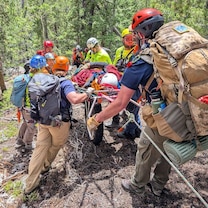
Stranded man was hiking for World Central Kitchen

• Aug 29, 11:51 AM

Woman found dead in her cubicle

• Aug 29, 7:16 PM

Army defends Arlington National Cemetery employee

• Aug 29, 12:46 PM

Foul play suspected in couple's disappearance

• Aug 29, 8:43 PM

Trump charged in Jan. 6 superseding indictment

• Aug 27, 6:25 PM

ABC News Live

24/7 coverage of breaking news and live events

• Our partners
• Our members
• Meet the team
• World Hospital Congress
• Geneva Sustainability Centre
• Knowledge exchange
• Association Leaders Circle
• Future of hospitals initiative
• Global Rare Paediatric Disease Network
• i-to-i Innovation Hub
• Harnessing Big Data SIG
• Telehealth: Navigating the future for hospitals SIG
• Leadership development
• IHF Leadership Model
• Healthcare leadership learning programme
• Outreach and partnerships
• Women in Leadership Special Interest Group
• Young Executive Leaders
• Articles and insights
• Newsletters
• Press & media
• Media partners
• Workshops and training
• Sustainability standards
• Sustainability Accelerator Tool (SAT)
• Carbon Emissions Learning Lab (CELL)
• Sustainability toolbox

Green care: Implementing sustainable practices in healthcare facilities (YEL 2024)

Date:   27 august 2024.

Authors: Omaira Valencia (Colombia), Maria Ribeiro da Cunha (Portugal), Amal Dahri (Morocco), Aban Gautam (Nepal), Abdur Rauf (Pakistan), Aline Mittag (Germany)

Reviewers: Hiba Al Naabi (YEL 2019, Accreditation head, the Royal Hospital, Oman), Olivier Costa (YEL 2022, Chief Medical Officer, Algemeen Ziekenhuis Sint-Maria Halle, Belgium), Carmen Menendez (Senior Project Officer, Geneva Sustainability Centre)

Introduction

The urgency of addressing climate change has never been more evident. The global community faces increasingly severe challenges, and without action, global temperatures could exceed the 1.5°C limit set by the Paris Agreement, potentially rising over 3°C by the century’s end (IPCC, 2021). The healthcare sector, responsible for about 5% of global emissions, is at the forefront of this crisis and must respond decisively to mitigate its impact (Karliner et al., 2019). Rapid warming, driven by unsustainable energy use, has profound public health implications, increasing heat-related illnesses, respiratory problems, and infectious diseases (Watts et al., 2018).

Adopting sustainable practices in healthcare is imperative. However, it requires concrete, actionable strategies across facilities. This article focuses on how the healthcare sector can reduce its environmental footprint while promoting public health by implementing sustainable practices. We propose four key areas intrinsically linked to global warming: energy efficiency, waste management, water conservation, and addressing climate change challenges for population health. These areas were selected as principal points where facilities can reduce their carbon footprint and align with global sustainability goals. Each area not only contributes to emission reductions but also strengthens the sector’s resilience against climate change impacts (World Health Organization, 2021).

Waste management

According to the World Health Organization (WHO), hospitals that implement sustainable waste management programmes can reduce their operating costs related to waste disposal by up to 20% (World Health Organization, 2018). Additionally, not only reduce their carbon footprint but also improve the safety and satisfaction of staff and patients, with a reported 15% increase in staff satisfaction in facilities with active recycling programmes (Watts et al., 2018).

Case study: Waste management reduction in healthcare facilities

Sustainable waste management in healthcare facilities is a global challenge that requires innovative and effective strategies. A notable example is Kaiser Permanente and Cleveland Clinic in the United States, which has achieved a 40% diversion of waste from landfills through recycling and composting programmes, as well as the implementation of a robust hazardous waste management programme (HPRC, 2022). However, these efforts are not exclusive to the United States. To better understand the practical steps involved in implementing a robust hazardous waste management programme, the following diagram outlines the key stages and actions taken by Kaiser Permanente (figure 1).

Figure 1: Sustainability programme cycle

When comparing waste management initiatives across different countries, similar approaches can be observed, with key differences in implementation. In Germany, the Freiburg University Hospital has managed to reduce hazardous waste by 35% by adopting advanced waste treatment technologies and strict segregation policies (Kaiser & Schmid, 2020). In Colombia, the Fundación Santa Fe de Bogotá has adopted Green Care initiatives that include reducing the use of single-use plastics (According to the national law) and implementing a recycling programme that has reduced waste sent to landfills by 25% over the past three years (Fundación Santa Fe de Bogotá, 2022). This success has been achieved through continuous staff education and collaboration with local recycling organizations. Unlike the United States and Colombia, where education and staff commitment are the main drivers, Germany has placed greater emphasis on technological investment to achieve its sustainability goals.

On the other hand, in Japan, hospitals have implemented a zero-waste approach, where more than 80% of materials are recycled or reused. This approach has been made possible through strong collaboration between the government, healthcare facilities, and local communities, resulting in a deeply ingrained culture of sustainability (Yamamoto & Kaneko, 2019).

Recommendations

• Conduct regular waste audits and establish baseline data for progress measurement.
• Train staff on new protocols and the importance of waste reduction.
• Develop partnerships for effective recycling and composting programmes.

Water conservation

Water conservation is increasingly critical in healthcare facilities, where resource efficiency directly impacts both operational costs and environmental sustainability. Hospitals around the world are implementing innovative strategies to reduce water consumption while maintaining high standards of care.

Case study: Water conservation

Cleveland Clinic in the USA has achieved a 30% reduction in water usage through advanced recycling systems and low-flow fixtures. Similarly, Rochdale Infirmary in the UK uses rainwater harvesting to supply non-potable water needs, complementing this with a rigorous leak detection programme that further minimizes wastage.

On the other hand, In India, Sir Ganga Ram Hospital has adopted a zero-discharge system, treating and reusing 100% of its wastewater for non-potable purposes. This approach not only conserves water but also reduces the hospital’s environmental footprint. Mount Elizabeth Hospital in Singapore has installed efficient cooling systems and sensor-activated faucets, significantly lowering water usage across the facility.

Hospital Universitario Austral in Argentina focuses on water-efficient landscaping and drip irrigation, which has led to substantial reductions in irrigation water demand. Mayo Clinic in the USA utilizes green roofs that collect rainwater for irrigation and employs advanced cooling tower management to minimize water waste. In Taiwan, Tzu Chi General Hospital has implemented water-efficient appliances and systems to reuse sterilization water, ensuring minimal waste. Table 1 shows some strategies used for implementing diverse water conservation strategies.

Table 1. Action steps for implementing water conservation techniques in healthcare facilities:

Reco mmendations

• Regularly audit plumbing systems and implement leak detection programmes.
• Promote the use of low-flow fixtures and water-efficient landscaping.
• Educate staff and the public on water conservation practices.

Energy efficiency and renewable energy

Energy and efficiency in healthcare institutions: german case study.

The report from the Ministry of Environment, Climate, and Energy of Baden-Württemberg (2016) provides case studies of successful implementation of energy efficiency measures in healthcare facilities in the region. Examples include the modernization of heating, ventilation, and air conditioning (HVAC) systems, the use of cogeneration systems, and the incorporation of renewable energies such as solar and biomass. These cases demonstrated not only significant cost savings but also improved comfort for patients and staff. Additionally, the Münch Foundation (2023) offers a handbook on actions and technologies for energy efficiency in hospitals. Key recommendations include regular energy audits, optimization of existing systems before investing in new technologies, and integration of energy management systems (EMS) that enable more effective monitoring and control of energy consumption. These approaches are essential to ensuring that investments in energy efficiency are cost-effective and sustainable in the long term.

Likewise, the Viamedica Foundation (2009) focuses on the adoption of renewable energy in German clinics, highlighting the use of solar energy and biomass. The energy demand in healthcare facilities and especially in hospitals is immense due to their constant availability, the high demand for technology.

In the adoption of these strategies, the following categories should be considered:

Energy efficiency

• Energy-saving behaviour : Encourage energy-saving behaviour among employees and patients. This requires a corporate culture that favours energy-saving actions and personnel to provide training on this topic. Examples include switching off lights and medical devices when not in use and installing water-saving fittings (MOH;2016).
• Lighting : Use LEDs, which require 90% less energy than conventional light bulbs and have a longer lifetime. Implement motion detectors for lighting control.
• Technical facilities : Replace and install high-efficiency pumps for heat and water transfer systems. Use heat recovery from waste heat to achieve energy savings.

Renewable energy

• Power source : Healthcare facilities should obtain electricity from renewable energy sources. Install solar systems on large hospital roof surfaces and consider adding battery storage systems. Choose green electricity suppliers to achieve the energy transition.
• Heat source : Utilize solar thermal, geothermal energy, biomass, or heat pumps. Integration into the regional heating network should also be considered.
• Develop a corporate culture that encourages energy-saving behaviours.
• Invest in energy-efficient technologies and infrastructure.
• Transition to renewable energy sources for both electricity and heat.

Addressing climate change challenges and improving population health

Climate change significantly worsens existing health issues, such as heat-related illnesses, respiratory problems, and infectious diseases, with an estimated 250,000 additional deaths per year expected between 2030 and 2050 (Watts et al., 2018). The health sector plays a vital role in addressing these challenges by reducing greenhouse gas emissions, enhancing infrastructure resilience, and implementing early warning systems for disease outbreaks (World Health Organization, 2018). Climate-related factors like heat waves, floods, and lack of clean water disproportionately affect vulnerable populations, driving the spread of diseases such as dengue, malaria, cholera, and tuberculosis (Ebi et al., 2018). Adressing these challenges requires urgent climate action and the adoption of integrated approaches like Ecosalud and One Health. Ecosalud broadly addresses the ecological determinants of health by integrating environmental, social, and economic factors, while One Health specifically focuses on the interconnectedness of human, animal, and environmental health, particularly concerning infectious diseases (Zinsstag et al., 2015).  Both approaches advocate for interdisciplinary collaboration and recognise the need for systems thinking to address complex health issues. In practice, Ecosalud and One Health can be integrated to provide a comprehensive approach to health that includes managing environmental determinants of health (Ecosalud) and preventing  zoonotic diseases (One Health) (figuere 2 and 3).

Figure 2: The one health approach

Adapted of hancock 1990; ecosystemic approach of health, jean lebel, idrc, 2003.

An example of the application of this approach is an intervention implemented in Girardot, Colombia, involved a step-by-step approach: (1) Assess ecological, biological, and social factors contributing to Aedes aegypti proliferation. (2) Develop a community-based intervention with insecticide-treated water container covers, window screens, and health education. (3) Implement the intervention in targeted areas, distributing materials and conducting home inspections. (4) Monitor and evaluate the impact using statistical models to compare dengue incidence before and after the intervention. (5)

Figure 3: The ecosystemic approach of health

Ensure sustainability by expanding coverage and maintaining community engagement to institutionalize the control measures. This intervention resulted in a reduction of dengue incidence by approximately 95 cases per year on average in the areas where the intervention was implemented (Quintero, 2020).

• Identify and assess vulnerabilities in communities and regions, health determinants and behavior challenges, health system capacities and identify multisectoral actors.
• Develop and implement targeted strategies in collaboration with various sectors.
• Monitor and evaluate the effectiveness of interventions regularly and scale-up models or effective strategies.

Addressing sustainability in healthcare is not just an option but a necessity. As young and future healthcare leaders, it is our responsibility to lead by example and implement sustainable practices within our organizations. By focusing on energy efficiency, waste management, water conservation, and addressing climate change challenges, we can significantly reduce the environmental footprint of healthcare facilities and promote public health.

The Young Executive Leaders (YEL) programme provides an excellent platform to share best practices, learn from each other, and drive the change needed for a sustainable future. Let us take decisive, effective action towards a more sustainable and resilient healthcare sector, leading the global effort to mitigate the effects of climate change.

• Ebi, K. L., Balbus, J. M., Luber, G., Bole, A., Crimmins, A., Glass, G., … & White-Newsome, J. L. (2018). Human Health. In Impacts, Risks, and Adaptation in the United States: The Fourth National Climate Assessment, Volume II. U.S. Global Change Research Program, 539–571. https://doi.org/10.7930/NCA4.2018.CH14
• Fundación Santa Fe de Bogotá. (2022). Informe de sostenibilidad 2022. Fundación Santa Fe de Bogotá. https://www.fundacionsantafedebogota.org.co/informe-de-sostenibilidad
• Intergovernmental Panel on Climate Change (IPCC). (2021). Climate Change 2021: The Physical Science Basis. Contribution of Working Group I to the Sixth Assessment Report of the Intergovernmental Panel on Climate Change. Cambridge University Press. https://www.ipcc.ch/report/ar6/wg1/
• Kaiser, S., & Schmid, P. (2020). Sustainable waste management in healthcare: A case study from Freiburg University Hospital. Environmental Science & Policy, 108, 95-101. https://doi.org/10.1016/j.envsci.2020.02.005
• Karliner, J., Slotterback, S., Boyd, R., Ashby, B., & Steele, K. (2019). Health care’s climate footprint: How the health sector contributes to the global climate crisis and opportunities for action. Health Care Without Harm. https://noharm-global.org/documents/health-care-climate-footprint-report
• Ministerium für Umwelt, Klima und Energiewirtschaft Baden-Württemberg. (2016). Energieeffizienz in Gesundheitseinrichtungen – Erfolgsbeispiele aus Baden-Württemberg. https://www.kea-bw.de/energieeffizienz-in-gesundheitseinrichtungen
• Quintero, J., Ronderos Pulido, N., Logan, J., Ant, T., Bruce, J., & Carrasquilla, G. (2020). Effectiveness of an intervention for Aedes aegypti control scaled-up under an inter-sectoral approach in a Colombian city hyper-endemic for dengue virus. PLoS ONE, 15(4), e0230486. https://doi.org/10.1371/journal.pone.0230486
• Stiftung Münch. (2023). Energieeffizienz im Krankenhaus – Handlungsleitfaden zu energiesparenden Ansätzen und Technologien. https://www.stiftung-muench.org/leitfaden-energieeffizienz.pdf
• Stiftung viamedica. (2009). Erneuerbare Energien und Energieeffizienz in deutschen Kliniken. https://www.viamedica-stiftung.de/prospekt_03.indd
• Watts, N., Amann, M., Arnell, N., Ayeb-Karlsson, S., Belesova, K., Berry, H., … & Costello, A. (2018). The 2018 report of The Lancet Countdown on health and climate change: Shaping the health of nations for centuries to come. The Lancet, 392(10163), 2479-2514. https://doi.org/10.1016/S0140-6736(18)32594-7
• World Health Organization. (2018). Climate change and health. Retrieved from https://www.who.int/news-room/fact-sheets/detail/climate-change-and-health
• World Health Organization. (2018). Safe management of wastes from health-care activities: A summary. World Health Organization. https://apps.who.int/iris/handle/10665/259491
• World Health Organization. (2021). COP26 Special Report on Climate Change and Health: The Health Argument for Climate Action. World Health Organization. https://www.who.int/publications/i/item/cop26-special-report
• Yamamoto, T., & Kaneko, S. (2019). Zero waste initiative in Japan’s healthcare sector: A case study analysis. Journal of Cleaner Production, 224, 451-460. https://doi.org/10.1016/j.jclepro.2019.03.256
• Zinsstag, J., Schelling, E., Waltner-Toews, D., & Tanner, M. (2015). One Health: The theory and practice of integrated health approaches. CABI. https://doi.org/10.1079/9781780643410.0000

Written by:

Victoria del pozo, news & insights, look into our latest....

Authors: Omaira Valencia (Colombia), Maria Ribeiro da Cunha (Portugal), Amal Dahri (Morocco), Aban Gautam (Nepal), Abdur Rauf (Pakistan), Aline Mittag...

Stanford Medicine: Using AI to make healthcare more human-centred

Artificial intelligence presents a unique opportunity to advance health and medicine globally – from diagnosing diseases sooner to accelerating research...

Value-based healthcare and outcome-based financing (YEL 2024)

Authors: Federico Umberto Mion (Group Chair), Vasco Dias (Group Co-Chair), Omar Zeyad (Group Co-Chair), Esther Ajowi, Daniel Burkhardt and Roshni...

The Geneva Sustainability Centre lands in South-East Asia

The CHI INNOVATE 2024 conference, held on 4 and 5 July 2024 in Singapore, had a simple pledge: An oath...

• Icon Twitter
• Subscribe to our newsletter

• Agriculture and Food Systems
• Biodiversity Conservation
• Climate Finance
• Conflict and Governance
• Gender and Social Inclusion
• Humanitarian Assistance
• Infrastructure
• Natural Climate Solutions
• Natural Resource Management
• Water and Sanitation
• Where We Work
• All Resources
• Climate Risk Management
• Climate Strategy Implementation
• Monitoring & Evaluation
• Tools & Support
• Engage with Us
• Photo Gallery
• Climate Strategy

July 2024 Newsletter Recap: Climate Resilience

Did you miss the Climatelinks July newsletter? We’ve got you covered. Please find a recap of the July ‘Climate Resilience’ theme below. You won’t want to miss this short list of top resources and blogs from the month. Subscribe to our newsletter today. Do you want to contribute to the Climatelinks community? Send us a resource, blog, or event.

Climate resilience can be generally defined as the capacity of a system to maintain function in the face of stresses imposed by climate change and to adapt the system to be better prepared for future climate impacts. One of the high-level goals in USAID’s 2022-2030 Climate Strategy is to improve the climate resilience of 500 million people.

Fresh Blog Posts

How usaid supports and scales climate resilience.

USAID's 2022-2030 Climate Strategy aims to support and scale the climate resilience of people, places, ecosystems, and livelihoods vulnerable to the impacts of climate change. The Agency is expanding access to climate information in decision making, increasing the climate resilience of key development sectors and services, and mainstreaming adaptation in plans and programs. It also employs nature-based solutions and engages the private sector in support of sustainable adaptation, including by mobilizing adaptation finance. 

Grassroots Project Jumpstarts Conservation Efforts in Mexican Countryside

Water scarcity and a hotter, drier climate were degrading the quality of life of residents in the small town of El Carrizal, Queretaro, Mexico . To address this, the town received a Peace Corps Small Project Assistance grant funded by USAID/Mexico to employ eco-techniques and technologies to advance environmentally conscious best practices and build climate resilience. The project constructed three rainwater collection cisterns, installed 10 solar hot water heaters, built two dry composting toilets, and created educational ecotourism signs. 

USAID’s Climate Strategy in Action: Cultivating Climate Resilience through Sustainable Ube Farming

In Palawan, Philippines , smallholder farmers face challenges to their livelihoods from the harsh realities of a changing climate. USAID’s Safe Water Activity is working to improve water security in water-stressed communities and support sustainable livelihood sources like ube farming. These efforts help both communities and the ecosystem become more resilient to climate change.  

Bridging the Gap with Parametric Insurance: A Path to Resilience in Developing Countries

With climate-related shocks and stresses increasing globally, economic losses due to natural hazards could skyrocket without efforts to invest in adaptation and build climate resilience. One potential solution is parametric insurance, which pays policyholders a predetermined amount based on the occurrence of a specific “trigger" event, like flooding or extreme heat. This allows the claims process to move faster and makes it less costly to manage.

Connecting Indonesia's First Large-Scale Floating Solar Plant to the Power Grid

The floating solar plant on the Citarum River in Indonesia is the largest floating solar plant in Southeast Asia and the third largest in the world. The USAID Sustainable Energy for Indonesia’s Advancing Resilience project helped integrate the plant into the country’s grid, allowing it to power 50,000 homes with clean energy. It is expected to reduce 3.1 million tons of carbon dioxide equivalent through 2035, which is comparable to preventing 3.4 billion pounds of coal from being burned. 

Empowering Communities: Climate Resilience Through Locally Led Adaptation

In the face of the climate crisis, local people and communities have emerged as frontline responders, both experiencing and addressing climate impacts. Locally Led Adaptation is an approach that supports local people, institutions, and networks to lead decisions on how, when, and where to adapt to the impacts of climate change. The USAID Climate Adaptation Support Activity has developed two new resources to help USAID and its partners further Locally Led Adaptation in practice.

New Resources

2024 gcc standard indicator handbook.

The 2024 Climate Change Standard Indicator Handbook has the latest USAID and Department of State standard indicators for climate change and development. It includes definition sheets that outline each indicator's linkage to a long-term outcome or impact and includes the proper unit of measure.

An Introduction to Assessing Climate Resilience in Smallholder Supply Chains

This resource, designed for medium- to high-level decision makers in food and beverage companies, offers a working definition of climate resilience, an actionable process guide, and sample indicator framework for diagnosing climate resilience in smallholder crop-focused supply chains. Ultimately, this guidance can help companies translate climate risk intelligence into practical, operational strategies to build supply chain resilience.

Climate Adaptation Learning Activity Fiscal Year 2024 Semi-Annual Report

The Climate Adaptation Knowledge and Learning Activity (CALA) works to improve the quality and effectiveness of climate adaptation efforts implemented by partners of USAID’s Bureau for Humanitarian Assistance. It does this by supporting the dissemination of learning and evidence related to climate adaptation programming. This Year 2 Semi-Annual Report provides a synopsis of progress made by the CALA Associate Award between October 1, 2023 and March 31, 2024, and offers a description of activities planned for the upcoming reporting period (April 1, 2024 – September 30, 2024).

Climate Risk Management Spotlight

Regional, sector, and country risk profiles and greenhouse gas emissions fact sheets.

Climate risk profiles (CRPs) summarize the key climate stressors and risks most relevant to a Mission’s objectives. These profiles can help promote climate resilience, which is imperative in addressing the multifaceted challenges posed by climate change. Check out the recently added Resilience and Food Security CRPs from USAID’s Bureau for Humanitarian Assistance. 

Call for Content

Share your events and resources or write a blog related to an upcoming monthly theme! Check out our upcoming themes to see if your climate work aligns:

• September and October: Just Energy Transition
• November: COP29
• 2024 Cross-cutting Themes: Systems Change and Locally Led Development

If your USAID-related climate change work relates to these themes, Climatelinks would love to feature your work and share your resources. Send us a resource or blog.

Strategic Objective

Climatelinks

Climatelinks is a global knowledge portal for USAID staff, implementing partners, and the broader community working at the intersection of climate change and international development. The portal curates and archives technical guidance and knowledge related to USAID’s work to help countries mitigate and adapt to climate change. 

Related Resources

Climate Strategy Webinar Series

Climate Risk Management Portal

Case Study: A Health Early Warning System to Reduce Extreme Heat Impacts in Senegal

Case Study: PEPFAR’s El Nino Response: Lessons Learned from Food Security and HIV/AIDS Crisis Funding

More on the blog, enhancing community resilience: addressing compound and cascading climate shocks.

• Dr. Jennifer Denno Cissé, Dr. Molly Hellmuth, Dr. Zarrar Khan

Building Effective Monitoring Networks: A Locally Led Approach to Fighting Climate Change

• Shannon Vasamsetti

The RISE Grants Challenge: Addressing Gender-based Violence in Climate and Environmental Contexts

• Jason Ocampo

Thank you for visiting nature.com. You are using a browser version with limited support for CSS. To obtain the best experience, we recommend you use a more up to date browser (or turn off compatibility mode in Internet Explorer). In the meantime, to ensure continued support, we are displaying the site without styles and JavaScript.

• View all journals
• Explore content
• About the journal
• Publish with us
• Sign up for alerts
• Open access
• Published: 26 August 2024

The genetic architecture of repeated local adaptation to climate in distantly related plants

• James R. Whiting   ORCID: orcid.org/0000-0001-8936-4991 1 ,
• Tom R. Booker 2 , 3 ,
• Clément Rougeux 1 ,
• Brandon M. Lind 1 , 3 ,
• Pooja Singh 1 , 4 , 5 ,
• Mengmeng Lu   ORCID: orcid.org/0000-0001-5023-3759 1 , 6 ,
• Kaichi Huang   ORCID: orcid.org/0000-0002-0378-5988 7 ,
• Michael C. Whitlock   ORCID: orcid.org/0000-0002-0782-1843 2 ,
• Sally N. Aitken   ORCID: orcid.org/0000-0002-2228-3625 3 ,
• Rose L. Andrew   ORCID: orcid.org/0000-0003-0099-8336 8 ,
• Justin O. Borevitz 9 ,
• Jeremy J. Bruhl 8 ,
• Timothy L. Collins 10 , 11 ,
• Martin C. Fischer   ORCID: orcid.org/0000-0002-1888-1809 12 ,
• Kathryn A. Hodgins   ORCID: orcid.org/0000-0003-2795-5213 13 ,
• Jason A. Holliday 14 ,
• Pär K. Ingvarsson   ORCID: orcid.org/0000-0001-9225-7521 15 ,
• Jasmine K. Janes   ORCID: orcid.org/0000-0002-4511-2087 16 , 17 , 18 ,
• Momena Khandaker 8 ,
• Daniel Koenig   ORCID: orcid.org/0000-0002-1037-5346 19 , 20 ,
• Julia M. Kreiner 7 , 21 ,
• Antoine Kremer   ORCID: orcid.org/0000-0002-3372-3235 22 ,
• Martin Lascoux   ORCID: orcid.org/0000-0003-1699-9042 23 ,
• Thibault Leroy   ORCID: orcid.org/0000-0003-2259-9723 24 ,
• Pascal Milesi   ORCID: orcid.org/0000-0001-8580-4291 23 ,
• Kevin D. Murray   ORCID: orcid.org/0000-0002-2466-1917 9 , 25 ,
• Tanja Pyhäjärvi   ORCID: orcid.org/0000-0001-6958-5172 26 , 27 ,
• Christian Rellstab   ORCID: orcid.org/0000-0002-0221-5975 28 ,
• Loren H. Rieseberg   ORCID: orcid.org/0000-0002-2712-2417 7 ,
• Fabrice Roux   ORCID: orcid.org/0000-0001-8059-5638 29 ,
• John R. Stinchcombe   ORCID: orcid.org/0000-0003-3349-2964 21 ,
• Ian R. H. Telford 8 ,
• Marco Todesco   ORCID: orcid.org/0000-0002-6227-4096 7 , 30 , 31 ,
• Jaakko S. Tyrmi 32 ,
• Baosheng Wang   ORCID: orcid.org/0000-0002-0934-1659 33 ,
• Detlef Weigel   ORCID: orcid.org/0000-0002-2114-7963 25 ,
• Yvonne Willi 34 ,
• Stephen I. Wright   ORCID: orcid.org/0000-0001-9973-9697 21 ,
• Lecong Zhou 14 &
• Sam Yeaman   ORCID: orcid.org/0000-0002-1706-8699 1  

Nature Ecology & Evolution ( 2024 ) Cite this article

1419 Accesses

5 Altmetric

Metrics details

• Evolutionary genetics
• Genetic variation

Closely related species often use the same genes to adapt to similar environments. However, we know little about why such genes possess increased adaptive potential and whether this is conserved across deeper evolutionary lineages. Adaptation to climate presents a natural laboratory to test these ideas, as even distantly related species must contend with similar stresses. Here, we re-analyse genomic data from thousands of individuals from 25 plant species as diverged as lodgepole pine and Arabidopsis (~300 Myr). We test for genetic repeatability based on within-species associations between allele frequencies in genes and variation in 21 climate variables. Our results demonstrate significant statistical evidence for genetic repeatability across deep time that is not expected under randomness, identifying a suite of 108 gene families (orthogroups) and gene functions that repeatedly drive local adaptation to climate. This set includes many orthogroups with well-known functions in abiotic stress response. Using gene co-expression networks to quantify pleiotropy, we find that orthogroups with stronger evidence for repeatability exhibit greater network centrality and broader expression across tissues (higher pleiotropy), contrary to the ‘cost of complexity’ theory. These gene families may be important in helping wild and crop species cope with future climate change, representing important candidates for future study.

Similar content being viewed by others

Large haploblocks underlie rapid adaptation in the invasive weed Ambrosia artemisiifolia

Massive haplotypes underlie ecotypic differentiation in sunflowers

Century-long timelines of herbarium genomes predict plant stomatal response to climate change

Is evolution repeatable? This question, captured by Stephen Jay Gould’s ‘replaying the tape of life’ metaphor 1 , has been the subject of decades of empirical research (reviewed in ref. 2 ). The answer appears to be context-dependent, with variation in repeatability among taxa, populations within species and genes in the genome, which leads to new questions about which evolutionary forces govern the continuum between identical parallel change and divergent responses 3 , 4 . The relative importance of deterministic versus stochastic and contingent explanations has been the subject of great interest and has been explored extensively at short evolutionary timescales among populations (for example, in stickleback 5 ) or closely related species (for example, Brassicaceae 6 , Arabidopsis spp. 7 and Heliconius spp. 8 ). These systems have highlighted predominant roles of the availability of common adaptive variation through shared inheritance 9 , 10 , 11 , gene flow 8 or recurrent mutation 12 . Experimental evolution has further emphasized the inverse associations between genetic repeatability and the complexity of adaptive trait architecture 13 . We know much less, however, about the processes and contingencies shaping genetic repeatability at much longer evolutionary distances or whether such distances impose hard limits on observing any repeatability at all. The Mc1r gene provides a textbook example of repeatability across deep time, driving adaptive colour polymorphism in distantly related vertebrates, from fish to mammoths 14 . Some have speculated that the widespread re-use of this gene is due to minimal interactions with other genes, facilitating its modification while incurring minimal pleiotropic disruption 15 . We have little understanding of whether the kinds of factors affecting repeatability for candidate genes such as Mc1r also generalize to drive repeatability at genome-wide scales or to adaptive phenotypes beyond simple traits such as colour.

Climatic variation across the species ranges of plants is a ubiquitous selection pressure among distantly related species, presenting a natural laboratory to study repeated adaptation. Such variation exerts strong selection pressure for local adaptation and genotypic responses 16 , demonstrable through common garden experiments or provenance trials and reciprocal transplants 17 . Numerous candidate genes for drought and thermal tolerance have been identified in, for example, Arabidopsis thaliana 18 , 19 , Panicum hallii 20 and conifers 21 . Plants may use a wide array of strategies to adapt to climate, including phenological shifts, such as flowering later to avoid frost or modification of structures, such as smaller leaves to mitigate the effect of air temperature in hotter climates 22 . While such studies have advanced our understanding of climate adaptation within individual species and have provided examples of a few individual candidate genes with evidence of adaptiveness in several species, there has been little combined analysis of whole-genome patterns across many species and large phylogenetic distances. There is reason to believe that phylogenetic constraints might exist for repeatability among plants, if, for example, mutational target size differs with genome size 23 . Alternatively, diverging lifestyles may limit common selection pressures or functional solutions 24 . Repeatability in adaptive genetic responses to climate across independently evolving species is expected if biological adaptation is limited to conserved functions, whereas a lack of repeatability might indicate highly polygenic, alternative adaptive strategies to the problem of climate adaptation 25 . The survival of plant populations challenged by anthropogenic climate change may depend on adaptation, which itself may depend on the maintenance of adaptive genetic variation within the metapopulation of a species through local adaptation 26 , 27 . Thus, studying repeatability of climate adaptation will give insights into the flexibility of such genetic responses, which will both deepen our understanding of evolution and help predict how species may respond to changes in the future.

Here, we analyse sequencing data from thousands of individuals from 25 plant species (Fig. 1 ) across a distribution spanning diverse biomes across four continents (Fig. 1a ) to investigate repeatability in the genetic basis of adaptation to climate variation. By processing all raw data through a common pipeline, we compiled by far the largest population genomics dataset to date in terms of phylogenetic breadth and sequencing effort to examine the phenomenon of repeated local adaptation across the genome. Our aims are to: (1) identify gene families that exhibit repeated evolutionary associations with climate across several species; (2) test whether genes driving repeated adaptation tend to fall within particular functional groups, suggestive of repeatability at the level of gene function; and (3) test whether properties of these gene families, specifically pleiotropy and duplication history, may facilitate their repeated evolution and significance for climate adaptation across the plant kingdom.

a , Sampling locations from all 29 datasets (25 species) and global annual mean temperature. b , An example of six bioclim variables across a single dataset with ten sampling locations from ref. 65 . c , An example for the same dataset showing how climate change variables were calculated, taking monthly climate data from the 1960s and 2010s and calculating the effect size of the difference between decades. d , The species tree derived from the OrthoFinder2 analysis for the 17 reference genomes used in this study; species where a reference genome assembly was used to map related species but that species was not included in analyses, are marked with asterisks. The reference genome assembly at each tip came from the species not listed in brackets and species listed in brackets below had their data mapped onto that reference genome. The age of high-confidence nodes is shown with values pulled from TimeTree (Extended Data Fig. 1 ). Species analysed here are placed according to the reference genome used and the reference’s position in the tree. e , f , The per genome distribution of the number of paralogues per orthogroup ( e ) and number of representative genomes per orthogroup ( f ) are depicted as stacked bars, with bar fill scaling from light-to-dark according to most- to least-statistically tractable value. Bars are ordered vertically in line with the tree in d . Ma, million years ago.

Results and discussion

Assembling datasets and defining orthology across species.

Twenty-nine datasets were downloaded from the NCBI sequencing read archive (SRA) or the EBI European nucleotide archive (ENA) repositories, covering 25 unique species (Supplementary Table 1 and Extended Data Fig. 1 ). These data were individual whole-genome sequencing (WGS), capture-based sequencing (CAPTURE) or pool-sequencing (POOL) data, each with a minimum of five sampling locations ( Methods gives full selection criteria). Raw reads were processed using a common single-nucleotide polymorphism (SNP)-calling pipeline (Supplementary Fig. 1 ) to minimize the influence of bioinformatic technical artefacts. The number of SNPs and individuals sampled per dataset ranged from 173,119 to 23,406,976 and 46 to ~1,300, respectively (Supplementary Table 1 ). To enable comparisons of several species (Fig. 1d ), we reconstructed orthology relationships using OrthoFinder2 (ref. 28 ) and classified genes into orthologous sets across species (orthogroups), which could include several copies of a gene in a given species due to gene duplication. In total, 44,861 orthogroups were classified, 14,328 were species-specific and 92.8% of all genes from all genomes were assigned to an orthogroup. Importantly, orthogroups were predominantly characterized by low rates of paralogy (Fig. 1e ), with rates of single-copy genes ranging from 39.8% to 62.4% (Supplementary Table 2 ) and high levels of presence across species (Fig. 1f ). From a statistical point of view, low paralogy is beneficial in aiding interpretation and comparison of genes among species and reducing confounding effects, whereas high presence across species increases statistical power to detect repeatability.

To identify genes with signatures of local adaptation within species, we performed genotype–environment association (GEA) scans by testing the association among population allele frequencies and population climatic variation (bioclim variables 1–19; Fig. 1b ) taken from worldclim (v.2.1, 2.5 arcmin resolution) 29 using non-parametric Kendall’s τ correlations ( Methods ). We also defined and quantified two variables that capture change in local climate (maximum temperature and precipitation) over the last 50 years. Briefly, these represent the effect size per sampling site of the difference between climate, quantified across a decade’s worth of data from either the 1960s or 2010s (example, in Fig. 1c ; Methods ). We then combined per SNP P values to calculate per gene P values using the weighted- Z analysis (WZA) 30 correcting for associations between SNP count and WZA variance. This WZA GEA method exhibits increased power and reduced error for identifying adaptive genes compared with other commonly used methods 30 .

To identify orthogroups with repeated signatures of association across several species, we applied PicMin 31 ( Methods ) across 8,470 orthogroups with at least 20 species represented for each of the 21 climate variables. These focal orthogroups were slightly more likely to include genes with stronger associations with climate relative to untested orthogroups (Supplementary Results 1 ). For orthogroups with several paralogues within a given species, we include the paralogue with the strongest evidence of association to test for repeatability after correction for multiple testing. This approach, therefore, tests for repeated adaptation driven by any member of a gene family.

Climate adaptation involves repeated gene re-use

Across all climate variables, we identified 141 repeatedly associated orthogroups (hereafter, RAOs) at a lenient false discovery rate (FDR) of 50%. These were made up of 108 unique orthogroups, with some showing significant hits for several climate variables, caused in part by covariance among climate variables. This set of RAOs represents an approximately threefold enrichment relative to expectations by chance, so although this list probably includes many individual RAOs that are false positives given the lenient threshold, it is highly unlikely to observe this many RAOs at FDR < 0.5 under a null model of no repeatability (1,000 random permutations, median expected number of RAOs was 36 across all variables, P  < 0.001; Fig. 2a,b ). Full details of randomizations and justification of thresholds are in Supplementary Methods 1 . In line with our first aim, these results demonstrate robust evidence for genetic repeatability across ~300 Myr of plant evolution and yield a suite of candidate orthogroups for further analysis. These 108 candidate RAOs will include false positives but these should only add noise to analyses of gene properties. A summary of statistical tests for all 141 RAOs is provided in Supplementary Table 3 .

a , b , Enrichment of the total ( a ) and unique ( b ) number of RAOs observed at FDR < 0.5 (red lines) relative to random permutations (distribution and mean dashed line). c , The number of orthogroups exhibiting significant repeatability at different FDR thresholds per climate variable. Details about the interpretation of FDR values are provided in the main text.

RAOs were observed across most climate variables, although the number of RAOs per climate variable and strength of statistical support varied. Generally, temperature variables exhibited more RAOs with stronger evidence of repeatability, in particular maximum temperature in the warmest month (Fig. 2c ). This indicates that the adaptive molecular response to temperature variation across plants may be more repeatable at the level of individual genes, compared with precipitation. This might reflect adaptive constraints underlying temperature adaptation or the added complexity of how precipitation interacts with soil to modulate drought effects. Variability in the number of RAOs identified across climate variables for a given species was not linked to inferred GEA power or relative niche breadth among species (as a proxy for selection variability) (Supplementary Results 2 and Supplementary Figs. 2 – 4 ). For downstream analyses, we focus on two sets of orthogroups: those with FDR < 0.5 to explore general trends in the distribution of RAOs among species and climate variables and to discuss specific candidate genes; and those with a PicMin P  < 0.005 (based on the top decile cutoff of strongest evidence of repeatability across all climate variables per orthogroup) within each climate variable to explore general properties of RAOs.

For RAOs (FDR < 0.5), we identified species driving the signature of repeatability on the basis of their per orthogroup P value ( Methods ). Visualizing the magnitude of these contributions by species and climate variables (Fig. 3a ) and among pairs of species (Fig. 3b ) demonstrates that no specific species, or cluster of species, contributes excessively to the repeatability signatures that we observe. In agreement, we failed to observe any evidence of phylogenetic signal of GEA results in our RAOs with respect to random orthogroups (Supplementary Results 3 and Extended Data Fig. 2 ). We reproduced Fig. 3a,b using RAOs detected at a more stringent FDR < 0.3 threshold and observed a comparable lack of phylogenetic signal (Extended Data Fig. 3 ). This shows that our identification of significant orthogroups is not driven by groups of closely related species but rather a signature observed broadly across the phylogenetic tree. This stands in contrast to expectations that repeatability declines as a function of relatedness among species 24 , 32 . Our result may be linked to the necessity of looking at conserved gene families, which may be less likely to have functionally diverged among species. In line with this, when repeating PicMin analyses only within Brassicaceae, we observed that statistical signals of repeatability tended to be stronger in our tested set of orthogroups (those with at least 20 species overall) relative to untested orthogroups with lower conservation (orthogroups with fewer than 20 species overall but including all Brassicaceae; Supplementary Results 4 and Supplementary Fig. 5 ).

a , b , Heatmaps show the contribution of individual species to orthogroup repeatability at FDR < 0.5 for different climate variables ( a ) and among pairs of species ( b ), with species ordered phylogenetically. In each case, the fill of each cell represents the proportion of orthogroups where a given species contributes towards the signature of repeatability based on its minimum GEA P value. c , Heatmap showing the number of times a species contributes towards repeatability for a given RAO (FDR < 0.5). In c , cell fill denotes the number of climate variables where a species contributes a low P value to a given RAO, with grey being 0. The vertical green line separates gymnosperms and angiosperms. Row-wise summations are shown as bars, where the blue bar shows the number of species associated with a given orthogroup (species n ) and the red bar shows the total number of species and climate variables (total n ). RAOs associated with a single climate variable only have a blue bar and those with stacked red bars are RAOs associated with multiple climate variables. The strongest statistical support for repeatability is also shown per orthogroup as −log 10 -transformed FDR. Only 73 RAOs with at least five contributing species are shown.

As an additional exploration into sources of variation within our repeatability analyses, we conducted leave-one-out cross-validations by removing each species and re-running PicMin (Supplementary Results 5 ). These analyses highlighted variation among species in terms of either increasing or decreasing the number of RAOs at FDR < 0.5 and <0.3. At FDR < 0.5, removing either Eucalyptus albens or E. sideroxylon reduced the number of RAOs the most, whereas removing Amaranthus tuberculatus caused the largest increase (Extended Data Fig. 4 ). Comparing these against features of the original SNP datasets indicated that reductions in RAOs were associated with removing datasets in which the sampling covered a larger amount of the global range of the species, geographically and in terms of climate breadth (Extended Data Fig. 4 ). Other factors, such as environmental similarity 5 , may also explain heterogeneity in repeatability among pairs of species (Fig. 3b ). The variability of dataset quality could confound signals among close relatives if, for example, they were sampled in different environments or to different extents of their ranges in our dataset.

Sixteen orthogroups were associated with repeatability across several climate variables. The orthogroup including the A. thaliana genes AT5G60100 ( PRR3 ) and AT5G02810 ( PRR7 ), with instrumental functional roles in circadian rhythm 33 and flowering time 34 , was repeatedly adaptive across 10 of 21 variables (most strongly with mean temperature in the dry quarter, FDR = 0.102; Extended Data Fig. 5 ) and across several variables within the same species (difference between red and blue bars in Fig. 3c ). The role of this gene family in circadian rhythm may contribute to its repeated association with several climate variables if these also vary with latitude. Another notable RAO includes a family of four genes encoding ubiquitin-related proteins: AT1G31340 ( RUB1 ), AT1G11980 ( RUB3 ), AT2G35635 ( UBQ7 ) , AT1G11970 , which was associated with six climate variables and most strongly with mean temperature (FDR = 0.051; Fig. 3c and Supplementary Table 3 ). The related-to-ubiquitin (RUB)-conjugation pathway has been implicated in the auxin response, embryo development and growth 35 . A summary of genes in RAOs that are associated with phenotypes known to be adaptive under climatic stress 36 is shown in Table 1 (full details of RAO gene contents in Supplementary Tables 4 – 6 ).

The functions of these genes reflect the expected responses to climatic variation, such as phenological avoidance of drought or frost through changes to flowering time or seed dormancy 22 or modification to root hair number and structure in response to temperature changes 37 . Changes to growth or stomatal function through hormone signalling 38 meanwhile may facilitate tolerance to drought by reducing water loss and genes associated with salt stress may be involved in surviving salt accumulation in soils due to aridity.

We found only a single RAO associated with our two climate change variables at FDR < 0.5; harbouring the A. thaliana genes AT5G53480 ( ATKPNB1 ), AT3G08943 and AT3G08947 . ATKPNB1 is sensitive to abscisic acid and is involved in drought tolerance through stomatal closure 39 . The few RAOs here may be due to the relatively short amount of time that our climate change variables are calculated over (~50 years) and the limited time to respond to selection subsequently, particularly in longer-lived species. Three species contributed to repeatability in this RAO (Supplementary Table 3 ), two of which are short-lived. However, given associations between our climate change variables and general bioclim variables (Extended Data Fig. 6 ), we cannot rule out contributions by longer-lived species.

Repeated adaptation across orthogroups with similar function

To examine repeatability beyond the gene level we characterized the functions of RAOs, to assess cases where several genes from within the same molecular pathway are used for adaptation across several species. Examples of ‘functional repeatability’ have been documented in adaptation to whole-genome duplication in Arabidopsis 40 and highland adaptation in maize 41 . To explore this phenomenon in accordance with our second aim, we used the STRING database 42 (v.11.5) to provide a network-based representation of protein–protein interactions (direct and indirect associations compiled from genomic context, experimental evidence such as co-expression and text-mining of literature) and tested whether RAOs formed networks with more interactions than expected ( Methods ). We grouped RAOs all together and into temperature- and precipitation-related groups and tested each group to see whether RAOs as a group contained genes that were more likely to interact with one another than random orthogroups.

Each group of RAOs tended to include more protein–protein interactions than random orthogroups and this was statistically significant for RAOs identified through precipitation variables, where ~2.4× more connections were observed than expected by chance (10,000 random permutations, average observed interactions was 19.06, expected number of interactions was 8.04, P  = 0.015) (Fig. 4a ). Gene ontology (GO) enrichment over the same groups of RAOs reflected this, as precipitation-related RAOs were highly enriched (hypergeometric test, one-tailed FDR < 0.1) for biological processes with clear adaptive roles (Fig. 4b,c and Supplementary Table 7 ). Orthogroups associated with ‘root hair tip’ were enriched across all RAOs (hypergeometric test, observed = 0.028, expected = 0.001, FDR = 0.046) and temperature RAOs were enriched for several processes, notably ‘regulation of photoperiodism, flowering’ (hypergeometric test, observed = 0.056, expected = 0.004, FDR = 0.016) and ‘brassinosteroid biosynthetic process’ (hypergeometric test, observed = 0.028, expected = 0.002, FDR = 0.099), which are known to be involved in thermotolerance 22 , 43 . These results suggest that independently identified RAOs contain genes involved in similar functional processes, which implies that repeated adaptation is also occurring beyond the level of the gene.

a , Mean number of STRING interactions within single-gene per orthogroup networks based on grouped RAOs (triangles) compared to results from permutation tests. Circles and lines represent the mean and 5/95% quantiles STRING interactions among 10,000 random gene sets sampled for single genes in the same way. The colour of circles shows the number of orthogroups in each group of RAOs. b , The network derived from all genes in precipitation-related RAOs, with orange highlighting which genes are members of four enriched GO terms within the same network. c , Enriched GO terms (FDR < 0.1) showing the number of contributing orthogroups from each species, with −log 10 -transformed FDR-adjusted significance shown as adjacent bars. GO terms are ordered on the y axis based on semantic similarity clustering, to group GO terms associated with similar genes together. Cell fill shows the number of orthogroups per species and GO term, with grey being 0.

The above patterns of enrichment may occur because a given adaptive response requires the coordinated modification of several functionally related genes in all species involved. Alternatively, this signal could also be driven by different subsets of functionally related genes contributing to adaptation in different subsets of species (for example, if genes A, B, C and D are functionally related, species 1, 2 and 3 adapt via genes A and D while species 4, 5 and 6 adapt via genes B and C). In either case, our results show that certain pathways or functional groups of genes are particularly important for adaptation to these climatic stressors, particularly with regards to adaptation to precipitation variation.

Repeatability is associated with increased pleiotropy

We next ask whether the gene families identified that contribute to repeated adaptation share particular characteristics with respect to their degree of pleiotropy. Pleiotropy is a fundamental attribute of a gene describing the number of traits it affects. On the basis of Fisher’s model of universal pleiotropy 44 , the ‘cost of complexity’ hypothesis 45 posits a reduced adaptive potential for genes with greater pleiotropy, as constraint increases with organismal ‘complexity’. In keeping with this, greater fitness consequences are predicted by the degree of pleiotropy in yeast 46 . However, empirical evidence from mice, nematodes and yeast suggests that this cost may be counteracted by a greater mutational effect size per trait observed for genes with greater pleiotropy 47 , 48 . In line with this, others 49 found genes repeatedly involved in stickleback adaptation exhibited elevated levels of pleiotropy.

To test the importance of pleiotropy by several definitions in our dataset, we used public databases of gene expression for A. thaliana and Medicago truncatula genes extracted from Expression Atlas 50 and ATTED-II 51 . We explored pleiotropy by two definitions: tissue specificity 52 and condition-independent co-expression with other genes 53 . Tissue specificity of gene expression is inversely associated with pleiotropy, has previously been linked to increased rates of evolution 54 and was estimated here according to the τ metric 55 (Fig. 5a ). The τ metric describes tissue specificity, the inverse of pleiotropy, so to avoid confusion we will describe changes to the breadth of expression, which we define as lower τ . Contrary to the cost of complexity prediction, we found that RAOs with the strongest evidence of repeatability were strongly associated with increased expression breadth (Stouffer’s Z , P  = 5.44 × 10 −4 ). Expression breadth also tended to decrease in subsets of orthogroups with increasingly weaker evidence of repeatability, such that orthogroups with the weakest evidence of repeatability were enriched for genes with high specificity (Stouffer’s Z , P  = 4.74 × 10 −6 ; Fig. 5b ).

a , An example of breadth of tissue expression. Each cell in the heatmap shows tissue-specific gene expression scaled by the maximum across all tissues for five genes, with their τ statistic as a bar. b , Stouffer’s Z calculated for orthogroups grouped into deciles on the basis of the strongest evidence of repeatability across all climate variables (green, P  < 0.05 more pleiotropic than expected; red, P  < 0.05 less pleiotropic than expected). c , An example network of 20 genes with four centrality measures calculated across nodes. Node size and colour (small-blue, low; large-red, high) denotes centrality by each metric. d , Stouffer’s Z for node degree and tissue specificity metrics within climate variables, focussing on orthogroups with at least one PicMin P  < 0.005. e , Non-parametric correlations of per orthogroup pleiotropy and duplication metrics, along with a randomized control variable. At, A. thaliana ; Mt, M. truncatula .

Alternatively, pleiotropic constraint can be considered as various node centrality statistics within a gene co-expression network (Fig. 5c ), where the ‘distance’ between two gene nodes is lower when co-expression of those genes increases (for example, across experimental treatments or tissue types). Co-expression centrality measures have been inversely linked to rate of evolution in several eukaryotic protein–protein networks and changes to genes with high centrality have a higher chance of being lethal 56 , 57 , indicative of evolutionary constraint. However, in contrast to these negative associations with evolvability, we observed clear positive associations between evidence of repeatability and co-expression centrality for node closeness, degree and strength across both co-expression networks (Fig. 5b ). Similar to results for expression breadth, centrality was significantly greater (Stouffer’s Z , P  < 0.05) in orthogroups with the strongest evidence of repeatability and significantly lower (Stouffer’s Z , P  < 0.05) in orthogroups with the weakest evidence. These clear trends across both specificity of tissue expression and co-expression networks highlight a robust association between increased pleiotropy and evidence of adaptive repeatability across all tested orthogroups. Associated measures of pleiotropy based on A. thaliana estimates for all orthogroups are included in Supplementary Table 8 .

The association we find between repeatability of local adaptation and increased pleiotropy stands in apparent contrast to previous findings of increased contributions to adaptation by genes with reduced pleiotropy 54 , 56 , 57 . This difference may arise because of the scale at which adaptation is occurring; here, we have focused on local adaptation, which involves a tension between migration and spatially divergent selection that tends to favour the contribution of alleles of large effect, as they can overcome migration swamping 25 , 58 . As the phenotypic effect size of mutations tends to increase with pleiotropy 47 , 48 , increased pleiotropy may therefore be favoured by natural selection during local adaptation. By contrast, when a species adapts to a temporal change in environment across its whole range, there is no tension between migration and selection and no further advantage for alleles of larger effect 25 . This may explain the reduced pleiotropy previously observed in rapidly evolving genes 54 , 56 , 57 . Our results suggest a robust impact of pleiotropy on local adaptation across several plant species, consistent with similar observations in stickleback 49 , ragweed 59 and A. thaliana 60 . It is unknown whether the association between pleiotropy and repeatability is monotonic or if intermediate pleiotropy promotes repeatability and extreme pleiotropy remains constraining, as suggested by refs. 49 , 60 . In the A. thaliana tissue specificity and node degree data, RAO sets were diminished for the least pleiotropic genes but also enriched for the most pleiotropic (Extended Data Fig. 7 ). It is important to make clear that we cannot rule out an association between repeatability and pleiotropy because of an increased likelihood of detecting large-effect alleles with GEA methods. A comparable analysis centred on global adaptation through selective sweeps could distinguish these, as selective sweep methods are similarly biased towards large-effect alleles but there is no assumption of a biological role for increased pleiotropy facilitating global adaptation at the species level 44 , 45 .

We were also interested in whether pleiotropy enrichment was limited to specific climate variables. We therefore repeated enrichment analyses for orthogroups exhibiting the strongest evidence of repeatability within climate variables (PicMin P  < 0.005) for tissue expression specificity and A. thaliana node degree (Fig. 5d ). Most of these sets of orthogroups exhibited elevated pleiotropy. Notably, orthogroups with the strongest evidence of repeatability associated with our climate change variables were highly enriched for pleiotropic genes by both measures (precipitation change—expression breadth P  = 0.0201, A. thaliana node degree P  = 0.0003; maximum temperature change—expression breadth P  = 0.0129, A. thaliana node degree P  = 0.0112). Given that these variables only capture environmental change over ~50 years, the genes with the strongest evidence of repeatability associated with these variables may be highly pleiotropic as a result of genes with greater effect sizes facilitating rapid adaptation to shifting fitness optima 61 .

Our orthogroup-level estimates of pleiotropy were also negatively associated with the number of gene duplication events within an orthogroup (Fig. 5e ). This was not an artefact of how per gene pleiotropy estimates were condensed to orthogroup-level estimates (Supplementary Results 6 ). Variability in gene duplication rate may also influence the likelihood of repeatability among gene families 62 . Indeed, we tended to see stronger evidence of repeatability in orthogroups with fewer duplication events, even when accounting for the effect of increased multiple-corrections (Extended Data Fig. 8 ). This negative association between duplications and repeatability is the opposite trend to that observed between conifer species by ref. 62 . This difference may stem from interactions between gene duplication and functional divergence over long periods of time. For example, between closely related species gene duplication may promote repeatability by alleviating functional constraints through neofunctionalization. However, across deep-time, gene families with higher rates of duplication may be expected to functionally diverge, inhibiting repeatability through a degradation in the common mapping of genotype to phenotype. Owing to inverse associations between duplication and pleiotropy estimates, however, it is difficult to disentangle these two properties of gene families (Supplementary Results 6 ).

Concluding remarks

Across plant species separated by >300 Myr of evolution, there is repeatability in the genetic basis of local adaptation to climate variation. The gene families identified in our analyses will be of substantial adaptive relevance as plants find themselves under increased climatic selection due to anthropogenic global change. We show that the adaptive responses to such changing selection involves conserved, core functional responses. We have also demonstrated that, contrary to expectations that pleiotropic constraint impedes adaptation, the genes identified as repeatedly adaptive bear signatures of increased pleiotropy. These results support the model of pleiotropy driving increasing phenotypic effect sizes and such large effects being a principal driver of local adaptation in the genome. Whether these results extend beyond the dominant biomes of boreal and temperate forest found in the Global North to species in the tropics and Global South is a question of great importance.

Dataset selection criteria

We selected 29 datasets covering 25 species from 21 studies 6 , 62 , 63 , 64 , 65 , 66 , 67 , 68 , 69 , 70 , 71 , 72 , 73 , 74 , 75 , 76 , 77 , 78 , 79 , 80 , 81 for which sequence data were available with WGS, POOL or CAPTURE (Supplementary Table 1 ). Such datasets provide broad genomic representation and maximize the resolution of the number of genes for each species. We limited our study to datasets with at least five populations distributed along latitudinal, longitudinal and/or altitudinal gradients. Here, the minimum number of populations was set to allow for a minimum baseline of statistical power for Kendall’s τ correlations between environment and allele frequency (see below). The list of included datasets is not exhaustive but rather was selected to achieve a desired number of approximately 20–30 species for which power to detect repeated adaptation has been demonstrated for the methods used here 82 . Datasets also had to provide locality information, either for individual samples or groups of individuals. Species were selected to include both gymnosperms and angiosperms, setting the most recent common ancestor of all species sampled at approximately 300 million years ago (Extended Data Fig. 1 ) 83 .

SNP-calling

We used two SNP-calling pipelines depending on whether sequencing data came from individuals (WGS and CAPTURE) or from pools of individuals (POOL). These pipelines were necessarily different but were based on similar approaches to reduce bioinformatic discrepancies between the data types. For all data types, raw fastq data were retrieved from either SRA or ENA. Accession codes for all data are provided in Supplementary Table 1 . The reference genomes used for each species, or closely related species if genomes were not available, are also in Supplementary Table 1 . SNP pipelines were designed to balance computational time and low false-positive rates 84 .

The pipeline for individual-based data was as follows, note that selfing and outcrossing species were processed using the same pipeline. Raw fastq files were cleaned and trimmed for adaptor sequences using fastp (v.0.20.1) 85 before being aligned against the reference genome using bwa-mem (v.0.7.17-r1188) 86 . BAM files were generated, sorted and indexed using samtools (v.1.16.1) 87 , skipping alignments with MAPQ < 10 (-q 10). We then collected quality metrics with Picard Tools (v.2.26.3) 88 based on alignment summary (CollectAlignmentSummaryMetrics), insert size metrics (CollectInsertSizeMetrics) and coverage (CollectWgsMetricsWithNonZeroCoverage). We then marked and removed duplicates using Picard’s MarkDuplicates and used AddOrReplaceReadGroups to amend read groups. In some cases, datasets split sequencing data from individual samples across several technical replicates, so we then merged BAM files within samples with Picard’s MergeSamFiles. We ran a realignment of the cleaned, merged BAM files by running the RealignerTargetCreator and IndelRealigner from the Genome Analysis Tool Kit (GATK v.3.8) 89 and repeated the aforementioned quality metrics on final BAM files. To identify SNPs, we generated genotype likelihoods using BCFtools 87 mpileup by specifying a minimum mapping quality of five for an alignment to be used and retained further annotation information such as allelic depth. From there, individual pileups were converted into SNP VCFs by using the BCFtools call programme. We set sample ploidy (-S) information to match the known ploidy of a species and called for genotype quality to be reported while excluding any group samples (-G -) information. Finally, we filtered raw VCF files with VCFtools 90 by removing sites with quality value below 30 (--minQ 30), Genotype quality below 20 (--minGQ 20), minimum read depth of 5 (--minDP 5), before finally retaining only biallelic (--max-alleles 2) genotypes present in >70% of individuals (--max-missing 0.7). For downstream analyses, we performed more filtering on the basis of minor allele frequency (maf) and minor allele count (mac), retaining only sites with maf > 0.05 and mac > 5, whichever was most stringent.

Pooled data were processed using a similarly structured workflow. Raw fastq files were cleaned and trimmed with fastp and aligned to references with bwa-mem using the additional flag to mark shorter split hits as secondary (-M). BAM files were generated, sorted and indexed using samtools, skipping alignments with MAPQ < 20 (-q 20) and bedfiles were generated from indexed BAM files using BEDtools (v.2.27.1) 91 . Duplicates were then marked and removed with MarkDuplicates before indel realignment was performed with Picard’s RealignerTargetCreator and IndelRealigner. SNP-calling was then performed using mpileup followed by the VarScan (v.2.4.2) mpileup2cns programme. Variants were called on the basis of minimum read depth of 8 (--in-coverage 8), a P value threshold of 0.05 (--p-value 0.05), a minimum frequency for calling homozygotes of 80% (--min-freq-for-hom 0.8), ignoring variants with >90% support on one strand (--strand-filter 1), minimum base quality at position of 20 (--min-avg-qual 20) and a minimum variant allele frequency of 0 (--min-var-freq = 0). To extract allele frequencies, pooled SNPs were converted to SNP tables using GATK (v.4.1.0.0) 92 VariantsToTable, splitting multi-allelic sites across multiple rows (--split-multi-allelic) and extracting the AF field. Final SNPTables for POOL data were filtered for indels, retaining only biallelic sites and a minor allele frequency cutoff of 0.05.

Orthology assignment

We grouped genes from each reference genome into orthogroups (sets of genes across species that are descended from a single gene in the last common ancestor 28 ) to facilitate comparisons among species. To construct orthogroups, we built proteomes for each reference genomes by extracting the protein sequence of the longest isoform for each gene using the AGAT (v.1.0.0) scripts agat_sp_keep_longest_isoform.pl and agat_sp_extract_sequences.pl. Proteomes were parsed as input to OrthoFinder2 (v.2.5.2) 28 using default settings. The species tree (Fig. 1d ) based on the reference genomes was inferred using all orthogroups where all genomes were represented ( n  = 5,003; Fig. 1f ) 93 , 94 .

Resulting orthogroups were then filtered for those that would yield the most statistical power, that is low rates of paralogy and high rates of species representation. Low rates of paralogy were necessary owing to multiple-comparison corrections performed among paralogues within species (see below), thus we removed a genome from an orthogroup if it had more than ten paralogues and retained only orthogroups with at least 20 representative species (this was dropped down to 19 species when analysing isothermality, as no GEA data were calculable for Eucalyptus magnificata for this variable). Of the 44,861 classified orthogroups, 8,470 were retained as high-quality for downstream analyses. The focal 8,470 high-quality orthogroups (20–25 species represented, maximum paralogue n per species of 10; Supplementary Fig. 6 ) covered 37.1%–61.6% of genes within each genome (Supplementary Table 2 ). The species tree from OrthoFinder was in good agreement with the species tree from TimeTree 83 (Supplementary Methods 2 and Supplementary Fig. 7 ). Only 355 orthogroups exhibited one-to-one orthology over 20 or more species, representing a substantial limitation of scope if only these were to be analysed.

Genotype–environment associations

For each unique latitude–longitude co-ordinate pair, we extracted bioclimatic variable (bioclim) data from the worldclim database (v.2.1) 29 at 2.5 arcmin resolution for all 19 bioclim variables. To describe recent climate change, we added two variables that quantified change in maximum temperature (tmax) and precipitation between all worldclim data collected monthly for the 1960s compared with the 2010s. As a measure of change, we estimated a non-parametric effect size between the distribution for each decade at each sampling location using the rstatix::wilcox_effsize() function 95 . Thus, a larger effect size is indicative of a greater change in recent climate (example shown in Fig. 1c ). We then calculated associations between individual allele frequencies and each of the 21 bioclim variables individually, without accounting for expected covariance among them (Supplementary Methods 3 ).

We first converted individual-based data into allele frequencies by combining individuals labelled as sampled from the same location and calculating per sampling site allele frequencies. These should not be considered as populations in the traditional population genetics sense, in that we do not assign populations on the basis of shared ancestry among individuals. In doing so, we trade off the risk of allele frequency sampling error when only a handful of individuals, or even a single individual, are sampled at a given location, against increased sampling power in downstream GEAs.

For each dataset, we combined per sampling location allele frequencies with our 21 climate variables and performed GEAs on the basis of non-parametric Kendall’s τ correlations (that is, no correction for population structure; justification of methodology is in Supplementary Methods 4 ). Each Kendalls’ τ correlation yields a P value for the correlation between allele frequency and environment. Because we are interested in repeatability at the gene level, we retained all SNPs within annotated gene boundaries (plus 500 base pair flanking regions) and converted P values to empirical P values (e P values: the rank of the P value divided by the number of P values) within each environmental variable. This yielded 21 uniform distributions of e P values across all SNPs for our 21 climate variables. To get gene-level GEA results, we combined evidence of all SNPs within each gene using the WZA 30 . This approach exploits the signal of elevated linkage among nearby SNPs within genes that is representative of local adaptation and has been shown to have similar or improved power and error relative to other GEA approaches including BayPass, RDA and LFMM 30 . The approach combines e P values from all SNPs within genes and flanks while weighting each SNP relative to its expected heterozygosity, resulting in a theoretically normal distribution of per gene Z -scores ( Z WZA ). We performed additional corrections to the Z WZA to account for heteroscedasiticity linked to variable SNP count per gene (Supplementary Methods 5 ).

If we had several datasets for an individual species ( A. thaliana , n  = 3; A. lyrata , n  = 2; A. halleri , n  = 2), we combined Z WZA P values within genes using Fisher’s approach, assuming each dataset represents an independent test of association between gene and environment, given datasets from the same species do not overlap spatially.

GEA repeatability testing

Because genes are not directly comparable among genomes, we combined per gene Z WZA e P values (e P value WZA ) with orthogroup assignments. Owing to low numbers of simple one-to-one orthogroups, we included species in orthogroups with a maximum of ten paralogues. For each species, we then retained the strongest signal of association (minimum e P value WZA ) within an orthogroup, correcting for the number of paralogues with a Dunn–Šidák correction, akin to Tippett’s method 96 . This approach of taking the strongest GEA among paralogues within the same orthogroup is based on the assumption that modification of any paralogue, rather than all paralogues, may be sufficient for adaptation if they are functionally similar 97 . This was preferable in contrast to simply combining evidence of association among all paralogues.

For each climate variable, we tested orthogroups with e P values WZA from at least 20 species for statistical clustering of low e P values WZA using PicMin 82 . PicMin was run in separate configurations depending on whether an orthogroup contained any of 20–25 species, with results combined at the end. Our null model for the among-species Tippett correction was that adaptation associated with an orthogroup is observed in one or no species. This test is performed by removing the minimum e P value WZA and testing each of the remaining n  − 1 e P values WZA against the expected probability density functions of n  − 1 random uniform draws. This generates a parametric P value for each observed e P value WZA based on how much lower the observed is relative to the beta expectation, which are combined according to Tippett’s method, that is taking the minimum P value corrected for the number of tests with a Dunn–Šidák correction and the expected correlation structure. This combined P value provides an estimate of the strength of evidence for the orthogroup contributing to repeated adaptation, with the rank of the minimum P value providing an estimation of the number of species driving the repeatability signature. A feature of PicMin under this null model is that as the number of species being tested increases, the multiple-comparison corrections applied increases to the point at which the distribution of PicMin P values across randomly distributed uniform P values is upwardly biased towards larger P values (Supplementary Fig. 8 ). This leads to an expected marginal loss of power. To address this, we simulated randomly distributed uniform P values from 20–25 species for 1,000,000 orthogroups and ran these through PicMin to generate an empirical distribution of PicMin P values under our random null model. We used this empirical null distribution to correct our observed PicMin P values using the qvalue::empPvals() function. For each climate variable analysed, the resulting corrected per orthogroup PicMin P values were FDR corrected and orthogroups with q  < 0.5 were considered as showing evidence of repeatability (RAOs). Justification of this threshold is in Supplementary Methods 1 .

STRING-db analyses

We tested for repeatability at a functional level by exploring functional interactions among RAOs. To do this, we took the A. thaliana genes from RAOs associated with each climate variable (FDR < 0.5) and asked whether these sets of genes were enriched for protein–protein interactions among orthogroups. We explored interactions within three groups: (1) all unique RAOs across all 21 climate variables; (2) unique RAOs related to temperature variables (bioclim 1–11 and tmax_clim_change); and (3) unique RAOs related to precipitation variables (bioclim 12–19 and prec_clim_change). To quantify interactions among genes, we used the STRING database 42 . We proposed that gene sets that were enriched for particular functions would include different orthogroups that included different, but functionally similar, genes that would interact with one another.

To explicitly measure interactions among orthogroups, as opposed to within, we first repeatedly sampled a single random gene from RAOs and quantified STRING interactions among these random single-gene per orthogroup gene sets. This was done to not count interactions among genes from the same orthogroup, which would be more likely to be functionally similar and potentially interact than random genes. Although this approach is conservative, single-copy genes are the most common in our orthogroups (Fig. 1e ). In the A. thaliana data used here, 58.5% of tested orthogroups were single copy, with two paralogues the next most common orthogroup size, so in most cases the loss of power incurred through randomly sampling a single gene should be minimal. With a single random gene per orthogroup, we then constructed the STRING network across these genes and counted the number of interactions across the network with medium or greater support (>0.4). We took the mean number of interactions across 1,000 networks (each time drawing a random single gene per orthogroup) for each of the three groups of RAOs as the ‘observed’ number of interactions (Fig. 4a ). We finally compared these observed values against 10,000 random draws, in which for each iteration we drew a random set of non-RAOs equivalent in size to each of the three groups. From this, we identified which sets of RAOs were associated with significantly more interactions among orthogroups than expected for random gene sets of equivalent size. An excess of interactions suggests that different orthogroups identified as repeatedly adaptive across different sets of species probably contain genes that are performing functionally similar roles but are not orthologous across species. Consequently, these networks may be particularly helpful at identifying more general biological processes that are associated with adaptation to climate if such processes are enriched within highly interactive networks.

We therefore asked what functions were enriched within all RAOs, temperature RAOs and precipitation RAOs. To do this, we collapsed GO assignments for all A. thaliana genes within a given orthogroup and removed duplicated GO terms. For example, if an orthogroup included two paralogues and paralogue 1 has GO terms GO1, GO2, GO3 whereas paralogue 2 has GO terms GO2, GO3 and GO4, the GO terms we retained for that orthogroup would be GO1, GO2, GO3 and GO4 (each once). This is important as our analysis is non-specific with regard to paralogues within orthogroups, so we cannot know which GO terms among paralogues may be relevant. We did this for all 8,470 tested orthogroups to produce a custom GO background and then assessed enrichment of GO terms within each set of RAOs. Enrichment of GO terms was determined on the basis of the hypergeometric expectation and P values were FDR corrected.

Orthogroup-level pleiotropy and repeatability

We estimated pleiotropy using two separate approaches: specificity of tissue expression and connectivity within co-expression networks. To calculate tissue specificity, we downloaded tissue expression data for A. thaliana from Expression Atlas 50 (accession no. E-MTAB-7978; ref. 98 ). This dataset comprises tissue expression (transcripts per million, TPM) across developmental stages, tissue types and subtissue type. Because we are interested specifically in specificity across different tissue types, we took the mean TPM across all developmental stages and subtissue types within the tissue type field. This resulted in mean TPM within each of the 23 tissue types (example in Fig. 5a ). The tissue specificity metric τ was calculated following ref. 55 as:

where, for a given gene, x i corresponds to the mean TPM for a given tissue type normalized by the maximum mean TPM across n tissue types. This yielded an estimate of τ for 30,074 A. thaliana genes. Of these, 25,831 could be matched to orthogroups and of these 15,472 were in the orthogroups tested for repeatability. To condense these to single orthogroup estimates, we converted τ estimates to rank-based e P values (least specific gives lowest e P value), took the lowest e P value within each orthogroup and corrected for the number of paralogues with a Dunn–Šidák correction. Finally, we transformed per orthogroup e P values to Z -scores with a mean of 0 and s.d. of 1 across all orthogroups. Alternative approaches were explored and are discussed in Supplementary Methods 6 .

As a complement to tissue specificity, we explored connectivity of genes in co-expression networks. We built two co-expression networks using co-expression data from ATTED-II 51 for A. thaliana and M. truncatula . Co-expression gene tables were downloaded for each species: A. thaliana , Ath-u.c3-0; M. truncatula , Mtr-u.c3-0. We discarded all edges with −5 <  Z  < 2.33 following the recommendations for significant negative or positive co-expression 51 . The A. thaliana network included 18,570 genes or 13,424 after retaining only genes in orthogroups tested for repeatability. Similarly, the M. truncatula network included 17,786 genes and 12,558 genes for the same groups. Networks were produced using the igraph package in R. Node betweenness and closeness were calculated using the estimate_betweenness() and closeness() functions, respectively. Node degree and strength were calculated as the number and absolute sum of edges respectively. The same approach was repeated for the co-expression network derived from M. truncatula . Orthogroup-level Z -scores were calculated for co-expression metrics as for expression specificity.

To assess how tissue expression specificity and co-expression centrality are associated with RAOs, we grouped orthogroups into deciles based on the strongest evidence for repeatability (minimum PicMin P value) observed for each orthogroup across all 21 climate variables. This was to rank orthogroups from ‘most repeatable’ to ‘least repeatable’ taking account of all tests performed. We then combined Z -scores within each decile based on Stouffer’s approach under a null hypothesis that if there is no association between repeatability and pleiotropy estimates, each decile should draw Z -scores randomly from the total distribution and yield Stouffer’s combined Z -scores of approximately 0. Stouffer’s Z -scores were finally converted to two-sided P values using the qnorm() function. We also performed the same analysis within each climate variable (Fig. 5d ).

Orthogroup-level duplication and repeatability

Information on duplications within orthogroups was obtained from the OrthoFinder2 outputs. We retained duplication events that had support >0.7 and occurred at nodes which included species that contributed GEA P values. This total number of duplications is therefore associated to the number of paralogues within orthogroups but counting the duplication events as opposed to the number of paralogues avoids counting the same duplication event several times. As well as counting the number of duplication events within each orthogroup gene tree, we also counted specifically the number of duplications that occur within species, that is all gene-tree tips downstream of the duplication node that include only the genome of a single species. We refer to these as species-specific duplications and were interested in these because of the potential for sub- and neo-functionalization to occur within species. We also quantified the number of single-copy genes per orthogroup. To examine associations of each of these duplication statistics with repeatability, we again split orthogroups into deciles on the basis of their strongest evidence of adaptive repeatability across the 21 climate variables and assessed how each per decile mean duplication metric varied from strongest to weakest evidence of repeatability.

To rule out the possibility that orthogroup structure and the number of paralogues drove associations between duplications and repeatability we used a randomization procedure (Supplementary Methods 7 ).

Reporting summary

Further information on research design is available in the Nature Portfolio Reporting Summary linked to this article.

Data availability

The SRA codes for all raw sequencing data are in Supplementary Table 1 . All VCFs and sample location data are available via Dryad at https://doi.org/10.5061/dryad.15dv41p57 (ref. 99 ).

Code availability

All scripts for SNP-calling and analyses are available and documented at https://github.com/JimWhiting91/RepAdapt and available via Zenodo at https://doi.org/10.5281/zenodo.12680122 (ref. 100 ).

Gould, S. J. Wonderful Life: The Burgess Shale and the Nature of History (WW Norton & Company, 1990).

Blount, Z. D., Lenski, R. E. & Losos, J. B. Contingency and determinism in evolution: replaying life’s tape. Science 362 , eaam5979 (2018).

Article   PubMed   Google Scholar  

Bolnick, D. I., Barrett, R. D. H., Oke, K. B., Rennison, D. J. & Stuart, Y. E. (Non)parallel evolution. Annu. Rev. Ecol. Evol. Syst. 49 , 303–330 (2018).

Article   Google Scholar  

Arendt, J. & Reznick, D. Convergence and parallelism reconsidered: what have we learned about the genetics of adaptation? Trends Ecol. Evol. 23 , 26–32 (2008).

Magalhaes, I. S. et al. Intercontinental genomic parallelism in multiple three-spined stickleback adaptive radiations. Nat. Ecol. Evol. 5 , 251–261 (2021).

Rellstab, C. et al. Genomic signatures of convergent adaptation to Alpine environments in three Brassicaceae species. Mol. Ecol. 29 , 4350–4365 (2020).

Article   CAS   PubMed   PubMed Central   Google Scholar  

Bohutínská, M. et al. Genomic basis of parallel adaptation varies with divergence in Arabidopsis and its relatives. Proc. Natl Acad. Sci. USA 118 , e2022713118 (2021).

Article   PubMed   PubMed Central   Google Scholar  

Montejo-Kovacevich, G. et al. Repeated genetic adaptation to altitude in two tropical butterflies. Nat. Commun. 13 , 4676 (2022).

Waters, J. M. & McCulloch, G. A. Reinventing the wheel? Reassessing the roles of gene flow, sorting and convergence in repeated evolution. Mol. Ecol. 30 , 4162–4172 (2021).

Konečná, V. et al. Parallel adaptation in autopolyploid Arabidopsis arenosa is dominated by repeated recruitment of shared alleles. Nat. Commun. 12 , 4979 (2021).

Louis, M. et al. Selection on ancestral genetic variation fuels repeated ecotype formation in bottlenose dolphins. Sci. Adv. 7 , eabg1245 (2021).

Zou, D. et al. Vulture genomes reveal molecular adaptations underlying obligate scavenging and low levels of genetic diversity. Mol. Biol. Evol. 38 , 3649–3663 (2021).

Long, A., Liti, G., Luptak, A. & Tenaillon, O. Elucidating the molecular architecture of adaptation via evolve and resequence experiments. Nat. Rev. Genet. 16 , 567–582 (2015).

Manceau, M., Domingues, V. S., Linnen, C. R., Rosenblum, E. B. & Hoekstra, H. E. Convergence in pigmentation at multiple levels: mutations, genes and function. Philos. Trans. R. Soc. Lond. B 365 , 2439–2450 (2010).

Article   CAS   Google Scholar  

Mundy, N. I. A window on the genetics of evolution: MC1R and plumage colouration in birds. Proc. Biol. Sci. 272 , 1633–1640 (2005).

CAS   PubMed   PubMed Central   Google Scholar  

Exposito-Alonso, M. et al. Natural selection on the Arabidopsis thaliana genome in present and future climates. Nature 573 , 126–129 (2019).

Article   CAS   PubMed   Google Scholar  

Lortie, C. J. & Hierro, J. L. A synthesis of local adaptation to climate through reciprocal common gardens. J. Ecol. 110 , 1015–1021 (2022).

Monroe, J. G. et al. Drought adaptation in Arabidopsis thaliana by extensive genetic loss-of-function. eLife 7 , e41038 (2018).

Exposito-Alonso, M. et al. Genomic basis and evolutionary potential for extreme drought adaptation in Arabidopsis thaliana . Nat. Ecol. Evol. 2 , 352–358 (2017).

Lovell, J. T. et al. The genomic landscape of molecular responses to natural drought stress in Panicum hallii . Nat. Commun. 9 , 5213 (2018).

MacLachlan, I. R. et al. Genome-wide shifts in climate-related variation underpin responses to selective breeding in a widespread conifer. Proc. Natl Acad. Sci. USA 118 , e2016900118 (2021).

James, M. E., Brodribb, T., Wright, I. J., Rieseberg, L. H. & Ortiz-Barrientos, D. Replicated evolution in plants. Annu. Rev. Plant Biol. 74 , 697–725 (2023).

Mei, W., Stetter, M. G., Gates, D. J., Stitzer, M. C. & Ross-Ibarra, J. Adaptation in plant genomes: bigger is different. Am. J. Bot. 105 , 16–19 (2018).

Bohutínská, M. & Peichel, C. L. Divergence time shapes gene reuse during repeated adaptation. Trends Ecol. Evol. 39 , 396–407 (2024).

Yeaman, S. Evolution of polygenic traits under global vs local adaptation. Genetics 220 , iyab134 (2022).

Anderson, J. & Song, B.-H. Plant adaptation to climate change—where are we? J. Syst. Evol. 58 , 533–545 (2020).

Christmas, M. J., Breed, M. F. & Lowe, A. J. Constraints to and conservation implications for climate change adaptation in plants. Conserv. Genet. 17 , 305–320 (2016).

Emms, D. M. & Kelly, S. OrthoFinder: phylogenetic orthology inference for comparative genomics. Genome Biol. 20 , 238 (2019).

Fick, S. E. & Hijmans, R. J. WorldClim 2: new 1‐km spatial resolution climate surfaces for global land areas. Int. J. Climatol. 37 , 4302–4315 (2017).

Booker, T. R., Yeaman, S., Whiting, J. R. & Whitlock, M. C. The WZA: a window-based method for characterizing genotype–environment association. Mol. Ecol. Resour. 24 , e13768 (2024).

Booker, T. R., Yeaman, S. & Whitlock, M. C. Using genome scans to identify genes used repeatedly for adaptation. Evolution 77 , 801–811 (2023).

Conte, G. L., Arnegard, M. E., Peichel, C. L. & Schluter, D. The probability of genetic parallelism and convergence in natural populations. Proc. Biol. Sci. 279 , 5039–5047 (2012).

PubMed   PubMed Central   Google Scholar  

Liu, T., Carlsson, J., Takeuchi, T., Newton, L. & Farré, E. M. Direct regulation of abiotic responses by the Arabidopsis circadian clock component PRR7. Plant J. 76 , 101–114 (2013).

Guan, J. et al. Genomic analyses of rice bean landraces reveal adaptation and yield related loci to accelerate breeding. Nat. Commun. 13 , 5707 (2022).

Bostick, M., Lochhead, S. R., Honda, A., Palmer, S. & Callis, J. Related to ubiquitin 1 and 2 are redundant and essential and regulate vegetative growth, auxin signaling, and ethylene production in Arabidopsis . Plant Cell 16 , 2418–2432 (2004).

Gray, S. B. & Brady, S. M. Plant developmental responses to climate change. Dev. Biol. 419 , 64–77 (2016).

Calleja-Cabrera, J., Boter, M., Oñate-Sánchez, L. & Pernas, M. Root growth adaptation to climate change in crops. Front. Plant Sci. 11 , 544 (2020).

Acharya, B. R. & Assmann, S. M. Hormone interactions in stomatal function. Plant Mol. Biol. 69 , 451–462 (2009).

Luo, Y. et al. An Arabidopsis homolog of importin β1 is required for ABA response and drought tolerance. Plant J. 75 , 377–389 (2013).

Bohutínská, M. et al. Novelty and convergence in adaptation to whole genome duplication. Mol. Biol. Evol. 38 , 3910–3924 (2021).

Wang, L. et al. Molecular parallelism underlies convergent highland adaptation of maize landraces. Mol. Biol. Evol. 38 , 3567–3580 (2021).

Szklarczyk, D. et al. The STRING database in 2021: customizable protein–protein networks, and functional characterization of user-uploaded gene/measurement sets. Nucleic Acids Res. 49 , D605–D612 (2021).

Li, N. et al. Plant hormone-mediated regulation of heat tolerance in response to global climate change. Front. Plant Sci. 11 , 627969 (2020).

Fisher, R. A. The Genetical Theory of Natural Selection Vol. 272 (Clarendon, 1930).

Orr, H. A. Adaptation and the cost of complexity. Evolution 54 , 13–20 (2000).

Cooper, T. F., Ostrowski, E. A. & Travisano, M. A negative relationship between mutation pleiotropy and fitness effect in yeast. Evolution 61 , 1495–1499 (2007).

Wang, Z., Liao, B.-Y. & Zhang, J. Genomic patterns of pleiotropy and the evolution of complexity. Proc. Natl Acad. Sci. USA 107 , 18034–18039 (2010).

Wagner, G. P. et al. Pleiotropic scaling of gene effects and the ‘cost of complexity’. Nature 452 , 470–472 (2008).

Rennison, D. J. & Peichel, C. L. Pleiotropy facilitates parallel adaptation in sticklebacks. Mol. Ecol. 31 , 1476–1486 (2022).

Papatheodorou, I. et al. Expression Atlas: gene and protein expression across multiple studies and organisms. Nucleic Acids Res. 46 , D246–D251 (2018).

Obayashi, T., Hibara, H., Kagaya, Y., Aoki, Y. & Kinoshita, K. ATTED-II v11: a plant gene coexpression database using a sample balancing technique by subagging of principal components. Plant Cell Physiol. 63 , 869–881 (2022).

Watanabe, K. et al. A global overview of pleiotropy and genetic architecture in complex traits. Nat. Genet. 51 , 1339–1348 (2019).

Proulx, S. R., Promislow, D. E. L. & Phillips, P. C. Network thinking in ecology and evolution. Trends Ecol. Evol. 20 , 345–353 (2005).

Mack, K. L., Phifer-Rixey, M., Harr, B. & Nachman, M. W. Gene expression networks across multiple tissues are associated with rates of molecular evolution in wild house mice. Genes 10 , 225 (2019).

Yanai, I. et al. Genome-wide midrange transcription profiles reveal expression level relationships in human tissue specification. Bioinformatics 21 , 650–659 (2005).

Hahn, M. W. & Kern, A. D. Comparative genomics of centrality and essentiality in three eukaryotic protein-interaction networks. Mol. Biol. Evol. 22 , 803–806 (2005).

Mähler, N. et al. Gene co-expression network connectivity is an important determinant of selective constraint. PLoS Genet. 13 , e1006402 (2017).

Lenormand, T. Gene flow and the limits to natural selection. Trends Ecol. Evol. 17 , 183–189 (2002).

Hämälä, T., Gorton, A. J., Moeller, D. A. & Tiffin, P. Pleiotropy facilitates local adaptation to distant optima in common ragweed ( Ambrosia artemisiifolia ). PLoS Genet. 16 , e1008707 (2020).

Frachon, L. et al. Intermediate degrees of synergistic pleiotropy drive adaptive evolution in ecological time. Nat. Ecol. Evol. 1 , 1551–1561 (2017).

Jain, K. & Stephan, W. Rapid adaptation of a polygenic trait after a sudden environmental shift. Genetics 206 , 389–406 (2017).

Yeaman, S. et al. Convergent local adaptation to climate in distantly related conifers. Science 353 , 1431–1433 (2016).

Kreiner, J. M. et al. Multiple modes of convergent adaptation in the spread of glyphosate-resistant Amaranthus tuberculatus . Proc. Natl Acad. Sci. USA 116 , 21076–21084 (2019).

Fischer, M. C. et al. Estimating genomic diversity and population differentiation—an empirical comparison of microsatellite and SNP variation in Arabidopsis halleri . BMC Genomics 18 , 69 (2017).

Kubota, S. et al. A genome scan for genes underlying microgeographic-scale local adaptation in a wild Arabidopsis species. PLoS Genet. 11 , e1005361 (2015).

Willi, Y., Fracassetti, M., Zoller, S. & Van Buskirk, J. Accumulation of mutational load at the edges of a species range. Mol. Biol. Evol. 35 , 781–791 (2018).

Mattila, T. M., Tyrmi, J., Pyhäjärvi, T. & Savolainen, O. Genome-wide analysis of colonization history and concomitant selection in Arabidopsis lyrata . Mol. Biol. Evol. 34 , 2665–2677 (2017).

Frachon, L. et al. A genomic map of climate adaptation in Arabidopsis thaliana at a micro-geographic scale. Front. Plant Sci. 9 , 967 (2018).

1001 Genomes Consortium. 1,135 genomes reveal the global pattern of polymorphism in Arabidopsis thaliana . Cell 166 , 481–491 (2016).

Wang, B. et al. Ancient polymorphisms contribute to genome-wide variation by long-term balancing selection and divergent sorting in Boechera stricta . Genome Biol. 20 , 126 (2019).

Koenig, D. et al. Long-term balancing selection drives evolution of immunity genes in Capsella . eLife 8 , e43606 (2019).

Murray, K. D. et al. Landscape drivers of genomic diversity and divergence in woodland Eucalyptus . Mol. Ecol. 28 , 5232–5247 (2019).

Todesco, M. et al. Massive haplotypes underlie ecotypic differentiation in sunflowers. Nature 584 , 602–607 (2020).

Yoder, J. B. et al. Genomic signature of adaptation to climate in Medicago truncatula . Genetics 196 , 1263–1275 (2014).

Gould, B. A. et al. Population genomics and climate adaptation of a C4 perennial grass, Panicum hallii (Poaceae). BMC Genomics 19 , 792 (2018).

Karunarathne, P., Zhou, Q., Lascoux, M. & Milesi, P. Hybridization mediated range expansion and climate change resilience in two conifers. Glob. Change Biol. https://doi.org/10.1111/gcb.17262 (2024).

Tyrmi, J. S. et al. Genomics of clinal local adaptation in Pinus sylvestris under continuous environmental and spatial genetic setting. G3 10 , 2683–2696 (2020).

Fahrenkrog, A. M. et al. Population genomics of the eastern cottonwood ( Populus deltoides ). Ecol. Evol. 7 , 9426–9440 (2017).

Wang, J. et al. A major locus controls local adaptation and adaptive life history variation in a perennial plant. Genome Biol. 19 , 72 (2018).

Holliday, J. A., Zhou, L., Bawa, R., Zhang, M. & Oubida, R. W. Evidence for extensive parallelism but divergent genomic architecture of adaptation along altitudinal and latitudinal gradients in Populus trichocarpa . New Phytol. 209 , 1240–1251 (2016).

Leroy, T. et al. Adaptive introgression as a driver of local adaptation to climate in European white oaks. New Phytol. 226 , 1171–1182 (2020).

Booker, T. R., Yeaman, S. & Whitlock, M. C. Using genome scans to identify genes used repeatedly for adaptation. Evolution 77 , 801–811 (2022).

Kumar, S., Stecher, G., Suleski, M. & Hedges, S. B. TimeTree: a resource for timelines, timetrees, and divergence times. Mol. Biol. Evol. 34 , 1812–1819 (2017).

Jasper, R. J. et al. Evaluating the accuracy of variant calling methods using the frequency of parent–offspring genotype mismatch. Mol. Ecol. Resour. 22 , 2524–2533 (2022).

Chen, S., Zhou, Y., Chen, Y. & Gu, J. fastp: an ultra-fast all-in-one FASTQ preprocessor. Bioinformatics 34 , i884–i890 (2018).

Li, H. Aligning sequence reads, clone sequences and assembly contigs with BWA-MEM. Preprint at https://doi.org/10.48550/arXiv.1303.3997 (2013).

Danecek, P. et al. Twelve years of SAMtools and BCFtools. Gigascience 10 , giab008 (2021).

Picard (Broad Institute, 2019); http://broadinstitute.github.io/picard/

DePristo, M. A. et al. A framework for variation discovery and genotyping using next-generation DNA sequencing data. Nat. Genet. 43 , 491–498 (2011).

Danecek, P. et al. The variant call format and VCFtools. Bioinformatics 27 , 2156–2158 (2011).

Quinlan, A. R. & Hall, I. M. BEDTools: a flexible suite of utilities for comparing genomic features. Bioinformatics 26 , 841–842 (2010).

Van der Auwera, G. A. & O’Connor, B. D. Genomics in the Cloud: Using Docker, GATK, and WDL in Terra (O’Reilly Media, 2020).

Emms, D. M. & Kelly, S. STAG: species tree inference from all genes. Preprint at bioRxiv https://doi.org/10.1101/267914 (2018).

Emms, D. M. & Kelly, S. STRIDE: Species tree root inference from gene duplication events. Mol. Biol. Evol. 34 , 3267–3278 (2017).

Kassambara, A. rstatix: Pipe-friendly framework for basic statistical tests. R package version 0.6.0 (2023).

Tippett, L. H. C. The Methods of Statistics: An Introduction Mainly for Workers in the Biological Sciences (Williams & Norgate, 1931).

Gabaldón, T. & Koonin, E. V. Functional and evolutionary implications of gene orthology. Nat. Rev. Genet. 14 , 360–366 (2013).

Mergner, J. et al. Mass-spectrometry-based draft of the Arabidopsis proteome. Nature 579 , 409–414 (2020).

Yeaman, S. & Whiting, J. R. The genetic architecture of repeated local adaptation to climate in distantly related plants. Dryad https://doi.org/10.5061/dryad.15dv41p57 (2024).

Whiting, J. R. et al. JimWhiting91/RepAdapt: Accepted Manuscript Release (v1.0.0). Zenodo https://doi.org/10.5281/zenodo.12680122 (2024).

Download references

Acknowledgements

We would like to thank O. Savolainen, T. Hämälä, T. Mitchell-Olds, D. Lowry, M. Kirst, P. Tiffin, S. Kubota and A. Widmer who were involved in the collection and preservation of data used in this study. Funding was provided by NSERC Discovery (RGPIN/03310-2023; S.Y.) and Alberta Innovates (212201729; S.Y.), with computational resources and support provided by the Digital Research Alliance of Canada (S.Y.).

Author information

Authors and affiliations.

Department of Biological Sciences, University of Calgary, Calgary, Alberta, Canada

James R. Whiting, Clément Rougeux, Brandon M. Lind, Pooja Singh, Mengmeng Lu & Sam Yeaman

Department of Zoology, Faculty of Science, University of British Columbia, Vancouver, British Colombia, Canada

Tom R. Booker & Michael C. Whitlock

Department of Forest and Conservation Sciences, Faculty of Forestry, University of British Columbia, Vancouver, British Columbia, Canada

Tom R. Booker, Brandon M. Lind & Sally N. Aitken

Aquatic Ecology and Evolution, Institute of Ecology and Evolution, University of Bern, Bern, Switzerland

Pooja Singh

EAWAG, Swiss Federal Institute of Aquatic Science and Technology, Kastanienbaum, Switzerland

Department of Biological Sciences, University of Notre Dame, Notre Dame, IN, USA

Mengmeng Lu

Department of Botany and Biodiversity Research Centre, University of British Columbia, Vancouver, British Columbia, Canada

Kaichi Huang, Julia M. Kreiner, Loren H. Rieseberg & Marco Todesco

School of Environmental and Rural Science, University of New England, Armidale, New South Wales, Australia

Rose L. Andrew, Jeremy J. Bruhl, Momena Khandaker & Ian R. H. Telford

Research School of Biology, Australian National University, Canberra, Australian Capital Territory, Australia

Justin O. Borevitz & Kevin D. Murray

Department of Planning and Environment, Queanbeyan, New South Wales, Australia

Timothy L. Collins

Department of Climate Change, Energy, the Environment and Water, Queanbeyan, New South Wales, Australia

ETH Zurich: Institute of Integrative Biology (IBZ), ETH Zurich, Zurich, Switzerland

Martin C. Fischer

School of Biological Sciences, Monash University, Melbourne, Victoria, Australia

Kathryn A. Hodgins

Department of Forest Resources and Environmental Conservation, Virginia Tech, Blacksburg, VA, USA

Jason A. Holliday & Lecong Zhou

Department of Plant Biology, Swedish University of Agricultural Sciences, Uppsala, Sweden

Pär K. Ingvarsson

Biology Department, Vancouver Island University, Nanaimo, British Columbia, Canada

Jasmine K. Janes

Department of Ecosystem Science and Management, University of Northern British Columbia, Prince George, British Columbia, Canada

Species Survival Commission, Orchid Specialist Group, IUCN North America, Washington, DC, USA

Department of Botany and Plant Sciences, University of California, Riverside, CA, USA

Daniel Koenig

Institute for Integrative Genome Biology, University of California, Riverside, CA, USA

Department of Ecology & Evolutionary Biology, University of Toronto, Toronto, Ontario, Canada

Julia M. Kreiner, John R. Stinchcombe & Stephen I. Wright

UMR BIOGECO, INRAE, Université de Bordeaux; 69 Route d’Arcachon, Cestas, France

Antoine Kremer

Program in Plant Ecology and Evolution, Department of Ecology and Genetics, Evolutionary Biology Centre and Science for Life Laboratory, Uppsala University, Uppsala, Sweden

Martin Lascoux & Pascal Milesi

GenPhySE, Université de Toulouse, INRAE, ENVT, Castanet Tolosan, France

Thibault Leroy

Department of Molecular Biology, Max Planck Institute for Biology Tübingen, Tübingen, Germany

Kevin D. Murray & Detlef Weigel

Department of Forest Sciences, University of Helsinki, Helsinki, Finland

Tanja Pyhäjärvi

Viikki Plant Science Centre, University of Helsinki, Helsinki, Finland

Swiss Federal Research Institute WSL, Birmensdorf, Switzerland

Christian Rellstab

Laboratoire des Interactions Plantes-Microbes-Environnement, Institut National de Recherche pour l’Agriculture, l’Alimentation et l’Environnement, CNRS, Université de Toulouse, Castanet-Tolosan, France

Fabrice Roux

Michael Smith Laboratories, University of British Columbia, Vancouver, British Columbia, Canada

Marco Todesco

Department of Biology, University of British Columbia, Kelowna, British Columbia, Canada

Department of Ecology and Genetics, University of Oulu, Oulu, Finland

Jaakko S. Tyrmi

South China National Botanical Garden, Guangzhou, China

Baosheng Wang

Department of Environmental Sciences, University of Basel, Basel, Switzerland

Yvonne Willi

You can also search for this author in PubMed   Google Scholar

Contributions

J.R.W. carried out the analysis and wrote the manuscript. S.Y. conceived the study, helped design the methods and analysis, and contributed to writing the manuscript. C. Rougeux organized the initial data collection and solicited contributions from collaborators. T.R.B. and M.C.W. helped design the methods. B.M.L., P.S., M. Lu and K. Huang contributed to bioinformatic methods and data processing. All other co-authors contributed data and edited the manuscript.

Corresponding authors

Correspondence to James R. Whiting or Sam Yeaman .

Ethics declarations

Competing interests.

The authors declare no competing interests.

Peer review

Peer review information.

Nature Ecology & Evolution thanks Magdalena Bohutinska and the other, anonymous, reviewer(s) for their contribution to the peer review of this work. Peer reviewer reports are available.

Additional information

Publisher’s note Springer Nature remains neutral with regard to jurisdictional claims in published maps and institutional affiliations.

Extended data

Extended data fig. 1 timetree phylogeny for the focal species studied here..

TimeTree 83 phylogeny for the species studied here. The phylogeny at the top provides estimates of node ages that are assessed across multiple studies that have dated the splits among clades. Asterisks denote cases where a substitute species was selected by TimeTree to be used as data on the target species was unavailable. The substituted species are not the same as those analysed in our study. Substituted species are: Amaranthus hybridus ( A. tuberculatus ); Eucalyptus erythrocorys ( E. albens ); Quercus rubra ( Quercus petraea ). A number of species are missing that were analysed, but congeneric representatives are shown (missing species: Helianthus petiolaris , E. magnificata , E. sideroxylon , Pinus contorta , Picea glauca x engelmannii ).

Extended Data Fig. 2 Lack of evidence for phylogenetic signal in RAOs.

The species tree that was used for phylogenetic tests is shown in panel A . Panel B shows the distribution of mean ‘K’ values across 1,000 random draws, each of 141 orthogroups. The mean ‘K’ observed in true RAOs is shown as a red line, and the mean of the random distribution is shown as a dashed black line.

Extended Data Fig. 3 Species contributions to repeatability in RAOs with PicMin FDR <0.3.

Heatmaps show the contribution of individual species to orthogroup repeatability at FDR < 0.3 for different climate variables ( A ) and among pairs of species ( B ), with species ordered phylogenetically. In each case, the fill of each cell represents the proportion of orthogroups where a given species contributes towards the signature of repeatability based on its minimum GEA p-value.

Extended Data Fig. 4 Leave-one-out cross validation results for PicMin repeatability analyses.

Panels A (FDR <0.5) and B (FDR <0.3) show stacked bars for RAOs identified when removing one species and testing the remaining 24, alongside the full 25 species dataset (vertical dashed line). The heatmap in C shows how the change in RAO number varied by species (LOO CV Change), alongside other features of species datasets including the breadth of sampling (geographically and climatically) relative to the total species range, and technical features related to genome sequencing and sample size (see Supplementary Results 5 ). The association between dataset features and the cross-validation results are shown as correlation coefficients in panel D . Negative correlation coefficients imply that removing datasets with lower dataset feature values increases the number of RAOs, and vice versa.

Extended Data Fig. 5 Summary of PicMin results for the orthogroup with the strongest evidence of repeatability across the most climate variables: OG0003045 ( Arabidopsis thaliana genes PRR3 and PRR7 ).

Heatmap in ( A ) shows the per species -log 10 -transformed GEA p-value for each species and climate variable. Note that isothermality is absent for Eucalyptus magnificata as there was no climate variation here. Alongside the heatmap, the -log 10 -transformed PicMin FDR values are shown, and rows are ordered according to the most significant to least significant. Individual GEA p-value vectors are plotted as histograms in ( B ), with the most significant in terms of PicMin FDR shown in top-left through to least significant in bottom-right.

Extended Data Fig. 6 Correlations between climate change variables and other bioclim variables across all individual datasets.

Each boxplot shows the non-parametric correlation coefficients calculated across all individual datasets (N = 29 biological replicates) between either precipitation climate change or maximum temperature climate change. Each box shows the median, quartiles, standard range (1.5 x IQR) and points show outliers beyond the standard range. Deviations from the central x = 0 are indicative of persistent association between a climate change variable and a given bioclim variable.

Extended Data Fig. 7 Decile enrichment of pleiotropy measures in orthogroups exhibiting strongest evidence of repeatability (PicMin p-value < 0.005).

Each pair of bars shows the proportion of Arabidopsis thaliana genes belonging to the relevant decile based on either specificity of tissue expression ( A ) or co-expression node degree ( B ), relative to the random expectation (red bars). Deciles are ordered 1-10 from least to most pleiotropic.

Extended Data Fig. 8 Associations between repeatability and gene duplication within orthogroups.

Panel A shows a simplified gene tree with 4 species (S1-S4), 3 duplications (D1-3), and 2 species-specific duplications (D2-3). Panel B shows depletion of duplications in orthogroups grouped according to their strongest evidence of repeatability. The mean duplication value is plotted for each repeatability decile. The black points and lines show a comparable analysis over 100 randomisations of all per gene ep-values WZA . The black point shows the mean duplication metric per decile and the lines show the maximum and minimum values across the 100 randomisations. Panel C shows duplication results exclusively looking at contributing species within RAOs, compared with species with low ep-values WZA (<0.1) within 10,000 draws of random orthogroup-climate sets. Lines show the observed mean relative to the distribution of random means, where green lines show permuted p-value < 0.05. The one-sided p-values for permutation tests = 0.153 (Mean Duplication N) and 0.035 (Mean Proportion of Duplicated Genes).

Supplementary information

Supplementary information.

Supplementary Methods 1–7, Results 1–7 and Figs. 1–12.

Reporting Summary

Peer review file, supplementary tables.

Supplementary Tables 1–8. Table legends are included with each sheet in the workbook.

Rights and permissions

Open Access This article is licensed under a Creative Commons Attribution 4.0 International License, which permits use, sharing, adaptation, distribution and reproduction in any medium or format, as long as you give appropriate credit to the original author(s) and the source, provide a link to the Creative Commons licence, and indicate if changes were made. The images or other third party material in this article are included in the article’s Creative Commons licence, unless indicated otherwise in a credit line to the material. If material is not included in the article’s Creative Commons licence and your intended use is not permitted by statutory regulation or exceeds the permitted use, you will need to obtain permission directly from the copyright holder. To view a copy of this licence, visit http://creativecommons.org/licenses/by/4.0/ .

Reprints and permissions

About this article

Cite this article.

Whiting, J.R., Booker, T.R., Rougeux, C. et al. The genetic architecture of repeated local adaptation to climate in distantly related plants. Nat Ecol Evol (2024). https://doi.org/10.1038/s41559-024-02514-5

Download citation

Received : 03 November 2023

Accepted : 22 July 2024

Published : 26 August 2024

DOI : https://doi.org/10.1038/s41559-024-02514-5

Share this article

Anyone you share the following link with will be able to read this content:

Sorry, a shareable link is not currently available for this article.

Provided by the Springer Nature SharedIt content-sharing initiative

Quick links

• Explore articles by subject
• Guide to authors
• Editorial policies

Sign up for the Nature Briefing newsletter — what matters in science, free to your inbox daily.

--> AGU