- Why Does Water Expand When It Freezes
- Gold Foil Experiment
- Faraday Cage
- Oil Drop Experiment
- Magnetic Monopole
- Why Do Fireflies Light Up
- Types of Blood Cells With Their Structure, and Functions
- The Main Parts of a Plant With Their Functions
- Parts of a Flower With Their Structure and Functions
- Parts of a Leaf With Their Structure and Functions
- Why Does Ice Float on Water
- Why Does Oil Float on Water
- How Do Clouds Form
- What Causes Lightning
- How are Diamonds Made
- Types of Meteorites
- Types of Volcanoes
- Types of Rocks

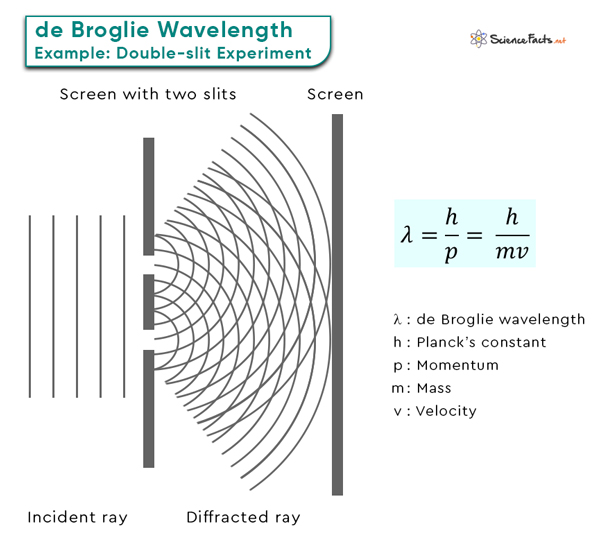
de Broglie Wavelength
The de Broglie wavelength is a fundamental concept in quantum mechanics that profoundly explains particle behavior at the quantum level. According to de Broglie hypothesis, particles like electrons, atoms, and molecules exhibit wave-like and particle-like properties.
This concept was introduced by French physicist Louis de Broglie in his doctoral thesis in 1924, revolutionizing our understanding of the nature of matter.
de Broglie Equation
A fundamental equation core to de Broglie hypothesis establishes the relationship between a particle’s wavelength and momentum . This equation is the cornerstone of quantum mechanics and sheds light on the wave-particle duality of matter. It revolutionizes our understanding of the behavior of particles at the quantum level. Here are some of the critical components of the de Broglie wavelength equation:
1. Planck’s Constant (h)
Central to this equation is Planck’s constant , denoted as “h.” Planck’s constant is a fundamental constant of nature, representing the smallest discrete unit of energy in quantum physics. Its value is approximately 6.626 x 10 -34 Jˑs. Planck’s constant relates the momentum of a particle to its corresponding wavelength, bridging the gap between classical and quantum physics.
2. Particle Momentum (p)
The second critical component of the equation is the particle’s momentum, denoted as “p”. Momentum is a fundamental property of particles in classical physics, defined as the product of an object’s mass (m) and its velocity (v). In quantum mechanics, however, momentum takes on a slightly different form. It is the product of the particle’s mass and its velocity, adjusted by the de Broglie wavelength.
The mathematical formulation of de Broglie wavelength is
We can replace the momentum by p = mv to obtain
The SI unit of wavelength is meter or m. Another commonly used unit is nanometer or nm.
This equation tells us that the wavelength of a particle is inversely proportional to its mass and velocity. In other words, as the mass of a particle increases or its velocity decreases, its de Broglie wavelength becomes shorter, and it behaves more like a classical particle. Conversely, as the mass decreases or velocity increases, the wavelength becomes longer, and the particle exhibits wave-like behavior. To grasp the significance of this equation, let us consider the example of an electron .
de Broglie Wavelength of Electron
Electrons are incredibly tiny and possess a minimal mass. As a result, when they are accelerated, such as when they move around the nucleus of an atom , their velocities can become significant fractions of the speed of light, typically ~1%.
Consider an electron moving at 2 x 10 6 m/s. The rest mass of an electron is 9.1 x 10 -31 kg. Therefore,
These short wavelengths are in the range of the sizes of atoms and molecules, which explains why electrons can exhibit wave-like interference patterns when interacting with matter, a phenomenon famously observed in the double-slit experiment.
Thermal de Broglie Wavelength
The thermal de Broglie wavelength is a concept that emerges when considering particles in a thermally agitated environment, typically at finite temperatures. In classical physics, particles in a gas undergo collision like billiard balls. However, particles exhibit wave-like behavior at the quantum level, including wave interference phenomenon. The thermal de Broglie wavelength considers the kinetic energy associated with particles due to their thermal motion.
At finite temperatures, particles within a system possess a range of energies described by the Maxwell-Boltzmann distribution. Some particles have relatively high energies, while others have low energies. The thermal de Broglie wavelength accounts for this distribution of kinetic energies. It helps to understand the statistical behavior of particles within a thermal ensemble.
Mathematical Expression
The thermal de Broglie wavelength (λ th ) is determined by incorporating both the mass (m) of the particle and its thermal kinetic energy (kT) into the de Broglie wavelength equation:
Here, k is the Boltzmann constant, and T is the temperature in Kelvin.
- de Broglie Wave Equation – Chem.libretexts.org
- de Broglie Wavelength – Spark.iop.org
- de Broglie Matter Waves – Openstax.org
- Wave Nature of Electron – Hyperphysics.phy-astr.gsu.edu
Article was last reviewed on Friday, October 6, 2023
Related articles

Leave a Reply Cancel reply
Your email address will not be published. Required fields are marked *
Save my name, email, and website in this browser for the next time I comment.
Popular Articles

Join our Newsletter
Fill your E-mail Address
Related Worksheets
- Privacy Policy
© 2024 ( Science Facts ). All rights reserved. Reproduction in whole or in part without permission is prohibited.
6.5 De Broglie’s Matter Waves
Learning objectives.
By the end of this section, you will be able to:
- Describe de Broglie’s hypothesis of matter waves
- Explain how the de Broglie’s hypothesis gives the rationale for the quantization of angular momentum in Bohr’s quantum theory of the hydrogen atom
- Describe the Davisson–Germer experiment
- Interpret de Broglie’s idea of matter waves and how they account for electron diffraction phenomena
Compton’s formula established that an electromagnetic wave can behave like a particle of light when interacting with matter. In 1924, Louis de Broglie proposed a new speculative hypothesis that electrons and other particles of matter can behave like waves. Today, this idea is known as de Broglie’s hypothesis of matter waves . In 1926, De Broglie’s hypothesis, together with Bohr’s early quantum theory, led to the development of a new theory of wave quantum mechanics to describe the physics of atoms and subatomic particles. Quantum mechanics has paved the way for new engineering inventions and technologies, such as the laser and magnetic resonance imaging (MRI). These new technologies drive discoveries in other sciences such as biology and chemistry.
According to de Broglie’s hypothesis, massless photons as well as massive particles must satisfy one common set of relations that connect the energy E with the frequency f , and the linear momentum p with the wavelength λ . λ . We have discussed these relations for photons in the context of Compton’s effect. We are recalling them now in a more general context. Any particle that has energy and momentum is a de Broglie wave of frequency f and wavelength λ : λ :
Here, E and p are, respectively, the relativistic energy and the momentum of a particle. De Broglie’s relations are usually expressed in terms of the wave vector k → , k → , k = 2 π / λ , k = 2 π / λ , and the wave frequency ω = 2 π f , ω = 2 π f , as we usually do for waves:
Wave theory tells us that a wave carries its energy with the group velocity . For matter waves, this group velocity is the velocity u of the particle. Identifying the energy E and momentum p of a particle with its relativistic energy m c 2 m c 2 and its relativistic momentum mu , respectively, it follows from de Broglie relations that matter waves satisfy the following relation:
where β = u / c . β = u / c . When a particle is massless we have u = c u = c and Equation 6.57 becomes λ f = c . λ f = c .
Example 6.11
How long are de broglie matter waves.
Depending on the problem at hand, in this equation we can use the following values for hc : h c = ( 6.626 × 10 −34 J · s ) ( 2.998 × 10 8 m/s ) = 1.986 × 10 −25 J · m = 1.241 eV · μ m h c = ( 6.626 × 10 −34 J · s ) ( 2.998 × 10 8 m/s ) = 1.986 × 10 −25 J · m = 1.241 eV · μ m
- For the basketball, the kinetic energy is K = m u 2 / 2 = ( 0.65 kg ) ( 10 m/s ) 2 / 2 = 32.5 J K = m u 2 / 2 = ( 0.65 kg ) ( 10 m/s ) 2 / 2 = 32.5 J and the rest mass energy is E 0 = m c 2 = ( 0.65 kg ) ( 2.998 × 10 8 m/s ) 2 = 5.84 × 10 16 J. E 0 = m c 2 = ( 0.65 kg ) ( 2.998 × 10 8 m/s ) 2 = 5.84 × 10 16 J. We see that K / ( K + E 0 ) ≪ 1 K / ( K + E 0 ) ≪ 1 and use p = m u = ( 0.65 kg ) ( 10 m/s ) = 6.5 J · s/m : p = m u = ( 0.65 kg ) ( 10 m/s ) = 6.5 J · s/m : λ = h p = 6.626 × 10 −34 J · s 6.5 J · s/m = 1.02 × 10 −34 m . λ = h p = 6.626 × 10 −34 J · s 6.5 J · s/m = 1.02 × 10 −34 m .
- For the nonrelativistic electron, E 0 = m c 2 = ( 9.109 × 10 −31 kg ) ( 2.998 × 10 8 m/s ) 2 = 511 keV E 0 = m c 2 = ( 9.109 × 10 −31 kg ) ( 2.998 × 10 8 m/s ) 2 = 511 keV and when K = 1.0 eV , K = 1.0 eV , we have K / ( K + E 0 ) = ( 1 / 512 ) × 10 −3 ≪ 1 , K / ( K + E 0 ) = ( 1 / 512 ) × 10 −3 ≪ 1 , so we can use the nonrelativistic formula. However, it is simpler here to use Equation 6.58 : λ = h p = h c K ( K + 2 E 0 ) = 1.241 eV · μ m ( 1.0 eV ) [ 1.0 eV+ 2 ( 511 keV ) ] = 1.23 nm . λ = h p = h c K ( K + 2 E 0 ) = 1.241 eV · μ m ( 1.0 eV ) [ 1.0 eV+ 2 ( 511 keV ) ] = 1.23 nm . If we use nonrelativistic momentum, we obtain the same result because 1 eV is much smaller than the rest mass of the electron.
- For a fast electron with K = 108 keV, K = 108 keV, relativistic effects cannot be neglected because its total energy is E = K + E 0 = 108 keV + 511 keV = 619 keV E = K + E 0 = 108 keV + 511 keV = 619 keV and K / E = 108 / 619 K / E = 108 / 619 is not negligible: λ = h p = h c K ( K + 2 E 0 ) = 1.241 eV · μm 108 keV [ 108 keV + 2 ( 511 keV ) ] = 3.55 pm . λ = h p = h c K ( K + 2 E 0 ) = 1.241 eV · μm 108 keV [ 108 keV + 2 ( 511 keV ) ] = 3.55 pm .
Significance
Check your understanding 6.11.
What is de Broglie’s wavelength of a nonrelativistic proton with a kinetic energy of 1.0 eV?
Using the concept of the electron matter wave, de Broglie provided a rationale for the quantization of the electron’s angular momentum in the hydrogen atom, which was postulated in Bohr’s quantum theory. The physical explanation for the first Bohr quantization condition comes naturally when we assume that an electron in a hydrogen atom behaves not like a particle but like a wave. To see it clearly, imagine a stretched guitar string that is clamped at both ends and vibrates in one of its normal modes. If the length of the string is l ( Figure 6.18 ), the wavelengths of these vibrations cannot be arbitrary but must be such that an integer k number of half-wavelengths λ / 2 λ / 2 fit exactly on the distance l between the ends. This is the condition l = k λ / 2 l = k λ / 2 for a standing wave on a string. Now suppose that instead of having the string clamped at the walls, we bend its length into a circle and fasten its ends to each other. This produces a circular string that vibrates in normal modes, satisfying the same standing-wave condition, but the number of half-wavelengths must now be an even number k , k = 2 n , k , k = 2 n , and the length l is now connected to the radius r n r n of the circle. This means that the radii are not arbitrary but must satisfy the following standing-wave condition:
If an electron in the n th Bohr orbit moves as a wave, by Equation 6.59 its wavelength must be equal to λ = 2 π r n / n . λ = 2 π r n / n . Assuming that Equation 6.58 is valid, the electron wave of this wavelength corresponds to the electron’s linear momentum, p = h / λ = n h / ( 2 π r n ) = n ℏ / r n . p = h / λ = n h / ( 2 π r n ) = n ℏ / r n . In a circular orbit, therefore, the electron’s angular momentum must be
This equation is the first of Bohr’s quantization conditions, given by Equation 6.36 . Providing a physical explanation for Bohr’s quantization condition is a convincing theoretical argument for the existence of matter waves.
Example 6.12
The electron wave in the ground state of hydrogen, check your understanding 6.12.
Find the de Broglie wavelength of an electron in the third excited state of hydrogen.
Experimental confirmation of matter waves came in 1927 when C. Davisson and L. Germer performed a series of electron-scattering experiments that clearly showed that electrons do behave like waves. Davisson and Germer did not set up their experiment to confirm de Broglie’s hypothesis: The confirmation came as a byproduct of their routine experimental studies of metal surfaces under electron bombardment.
In the particular experiment that provided the very first evidence of electron waves (known today as the Davisson–Germer experiment ), they studied a surface of nickel. Their nickel sample was specially prepared in a high-temperature oven to change its usual polycrystalline structure to a form in which large single-crystal domains occupy the volume. Figure 6.19 shows the experimental setup. Thermal electrons are released from a heated element (usually made of tungsten) in the electron gun and accelerated through a potential difference Δ V , Δ V , becoming a well-collimated beam of electrons produced by an electron gun. The kinetic energy K of the electrons is adjusted by selecting a value of the potential difference in the electron gun. This produces a beam of electrons with a set value of linear momentum, in accordance with the conservation of energy:
The electron beam is incident on the nickel sample in the direction normal to its surface. At the surface, it scatters in various directions. The intensity of the beam scattered in a selected direction φ φ is measured by a highly sensitive detector. The detector’s angular position with respect to the direction of the incident beam can be varied from φ = 0 ° φ = 0 ° to φ = 90 ° . φ = 90 ° . The entire setup is enclosed in a vacuum chamber to prevent electron collisions with air molecules, as such thermal collisions would change the electrons’ kinetic energy and are not desirable.
When the nickel target has a polycrystalline form with many randomly oriented microscopic crystals, the incident electrons scatter off its surface in various random directions. As a result, the intensity of the scattered electron beam is much the same in any direction, resembling a diffuse reflection of light from a porous surface. However, when the nickel target has a regular crystalline structure, the intensity of the scattered electron beam shows a clear maximum at a specific angle and the results show a clear diffraction pattern (see Figure 6.20 ). Similar diffraction patterns formed by X-rays scattered by various crystalline solids were studied in 1912 by father-and-son physicists William H. Bragg and William L. Bragg . The Bragg law in X-ray crystallography provides a connection between the wavelength λ λ of the radiation incident on a crystalline lattice, the lattice spacing, and the position of the interference maximum in the diffracted radiation (see Diffraction ).
The lattice spacing of the Davisson–Germer target, determined with X-ray crystallography, was measured to be a = 2.15 Å . a = 2.15 Å . Unlike X-ray crystallography in which X-rays penetrate the sample, in the original Davisson–Germer experiment, only the surface atoms interact with the incident electron beam. For the surface diffraction, the maximum intensity of the reflected electron beam is observed for scattering angles that satisfy the condition n λ = a sin φ n λ = a sin φ (see Figure 6.21 ). The first-order maximum (for n = 1 n = 1 ) is measured at a scattering angle of φ ≈ 50 ° φ ≈ 50 ° at Δ V ≈ 54 V , Δ V ≈ 54 V , which gives the wavelength of the incident radiation as λ = ( 2.15 Å ) sin 50 ° = 1.64 Å . λ = ( 2.15 Å ) sin 50 ° = 1.64 Å . On the other hand, a 54-V potential accelerates the incident electrons to kinetic energies of K = 54 eV . K = 54 eV . Their momentum, calculated from Equation 6.61 , is p = 2.478 × 10 −5 eV · s / m . p = 2.478 × 10 −5 eV · s / m . When we substitute this result in Equation 6.58 , the de Broglie wavelength is obtained as
The same result is obtained when we use K = 54 eV K = 54 eV in Equation 6.61 . The proximity of this theoretical result to the Davisson–Germer experimental value of λ = 1.64 Å λ = 1.64 Å is a convincing argument for the existence of de Broglie matter waves.
Diffraction lines measured with low-energy electrons, such as those used in the Davisson–Germer experiment, are quite broad (see Figure 6.20 ) because the incident electrons are scattered only from the surface. The resolution of diffraction images greatly improves when a higher-energy electron beam passes through a thin metal foil. This occurs because the diffraction image is created by scattering off many crystalline planes inside the volume, and the maxima produced in scattering at Bragg angles are sharp (see Figure 6.22 ).
Since the work of Davisson and Germer, de Broglie’s hypothesis has been extensively tested with various experimental techniques, and the existence of de Broglie waves has been confirmed for numerous elementary particles. Neutrons have been used in scattering experiments to determine crystalline structures of solids from interference patterns formed by neutron matter waves. The neutron has zero charge and its mass is comparable with the mass of a positively charged proton. Both neutrons and protons can be seen as matter waves. Therefore, the property of being a matter wave is not specific to electrically charged particles but is true of all particles in motion. Matter waves of molecules as large as carbon C 60 C 60 have been measured. All physical objects, small or large, have an associated matter wave as long as they remain in motion. The universal character of de Broglie matter waves is firmly established.
Example 6.13
Neutron scattering.
We see that p 2 c 2 ≪ E 0 2 p 2 c 2 ≪ E 0 2 so K ≪ E 0 K ≪ E 0 and we can use the nonrelativistic kinetic energy:
Kinetic energy of ideal gas in equilibrium at 300 K is:
We see that these energies are of the same order of magnitude.
Example 6.14
Wavelength of a relativistic proton, check your understanding 6.13.
Find the de Broglie wavelength and kinetic energy of a free electron that travels at a speed of 0.75 c .
This book may not be used in the training of large language models or otherwise be ingested into large language models or generative AI offerings without OpenStax's permission.
Want to cite, share, or modify this book? This book uses the Creative Commons Attribution License and you must attribute OpenStax.
Access for free at https://openstax.org/books/university-physics-volume-3/pages/1-introduction
- Authors: Samuel J. Ling, Jeff Sanny, William Moebs
- Publisher/website: OpenStax
- Book title: University Physics Volume 3
- Publication date: Sep 29, 2016
- Location: Houston, Texas
- Book URL: https://openstax.org/books/university-physics-volume-3/pages/1-introduction
- Section URL: https://openstax.org/books/university-physics-volume-3/pages/6-5-de-broglies-matter-waves
© Jul 23, 2024 OpenStax. Textbook content produced by OpenStax is licensed under a Creative Commons Attribution License . The OpenStax name, OpenStax logo, OpenStax book covers, OpenStax CNX name, and OpenStax CNX logo are not subject to the Creative Commons license and may not be reproduced without the prior and express written consent of Rice University.

Photons and Matter Waves
De Broglie’s Matter Waves
Samuel J. Ling; Jeff Sanny; and William Moebs
Learning Objectives
By the end of this section, you will be able to:
- Describe de Broglie’s hypothesis of matter waves
- Explain how the de Broglie’s hypothesis gives the rationale for the quantization of angular momentum in Bohr’s quantum theory of the hydrogen atom
- Describe the Davisson–Germer experiment
- Interpret de Broglie’s idea of matter waves and how they account for electron diffraction phenomena
Compton’s formula established that an electromagnetic wave can behave like a particle of light when interacting with matter. In 1924, Louis de Broglie proposed a new speculative hypothesis that electrons and other particles of matter can behave like waves. Today, this idea is known as de Broglie’s hypothesis of matter waves . In 1926, De Broglie’s hypothesis, together with Bohr’s early quantum theory, led to the development of a new theory of wave quantum mechanics to describe the physics of atoms and subatomic particles. Quantum mechanics has paved the way for new engineering inventions and technologies, such as the laser and magnetic resonance imaging (MRI). These new technologies drive discoveries in other sciences such as biology and chemistry.

and the rest mass energy is

Significance We see from these estimates that De Broglie’s wavelengths of macroscopic objects such as a ball are immeasurably small. Therefore, even if they exist, they are not detectable and do not affect the motion of macroscopic objects.
Check Your Understanding What is de Broglie’s wavelength of a nonrelativistic proton with a kinetic energy of 1.0 eV?

This equation is the first of Bohr’s quantization conditions, given by (Figure) . Providing a physical explanation for Bohr’s quantization condition is a convincing theoretical argument for the existence of matter waves.

The Electron Wave in the Ground State of Hydrogen Find the de Broglie wavelength of an electron in the ground state of hydrogen.

Significance We obtain the same result when we use (Figure) directly.
Check Your Understanding Find the de Broglie wavelength of an electron in the third excited state of hydrogen.

Experimental confirmation of matter waves came in 1927 when C. Davisson and L. Germer performed a series of electron-scattering experiments that clearly showed that electrons do behave like waves. Davisson and Germer did not set up their experiment to confirm de Broglie’s hypothesis: The confirmation came as a byproduct of their routine experimental studies of metal surfaces under electron bombardment.

Diffraction lines measured with low-energy electrons, such as those used in the Davisson–Germer experiment, are quite broad (see (Figure) ) because the incident electrons are scattered only from the surface. The resolution of diffraction images greatly improves when a higher-energy electron beam passes through a thin metal foil. This occurs because the diffraction image is created by scattering off many crystalline planes inside the volume, and the maxima produced in scattering at Bragg angles are sharp (see (Figure) ).

Neutron Scattering Suppose that a neutron beam is used in a diffraction experiment on a typical crystalline solid. Estimate the kinetic energy of a neutron (in eV) in the neutron beam and compare it with kinetic energy of an ideal gas in equilibrium at room temperature.

Kinetic energy of ideal gas in equilibrium at 300 K is:

We see that these energies are of the same order of magnitude.
Significance Neutrons with energies in this range, which is typical for an ideal gas at room temperature, are called “thermal neutrons.”
Wavelength of a Relativistic Proton In a supercollider at CERN, protons can be accelerated to velocities of 0.75 c . What are their de Broglie wavelengths at this speed? What are their kinetic energies?

Check Your Understanding Find the de Broglie wavelength and kinetic energy of a free electron that travels at a speed of 0.75 c .

- De Broglie’s hypothesis of matter waves postulates that any particle of matter that has linear momentum is also a wave. The wavelength of a matter wave associated with a particle is inversely proportional to the magnitude of the particle’s linear momentum. The speed of the matter wave is the speed of the particle.
- De Broglie’s concept of the electron matter wave provides a rationale for the quantization of the electron’s angular momentum in Bohr’s model of the hydrogen atom.
- In the Davisson–Germer experiment, electrons are scattered off a crystalline nickel surface. Diffraction patterns of electron matter waves are observed. They are the evidence for the existence of matter waves. Matter waves are observed in diffraction experiments with various particles.
Conceptual Questions
Which type of radiation is most suitable for the observation of diffraction patterns on crystalline solids; radio waves, visible light, or X-rays? Explain.
X-rays, best resolving power

If an electron and a proton are traveling at the same speed, which one has the shorter de Broglie wavelength?
If a particle is accelerating, how does this affect its de Broglie wavelength?
Why is the wave-like nature of matter not observed every day for macroscopic objects?
negligibly small de Broglie’s wavelengths
What is the wavelength of a neutron at rest? Explain.
Why does the setup of Davisson–Germer experiment need to be enclosed in a vacuum chamber? Discuss what result you expect when the chamber is not evacuated.
to avoid collisions with air molecules
At what velocity will an electron have a wavelength of 1.00 m?

What is the de Broglie wavelength of an electron that is accelerated from rest through a potential difference of 20 keV?
What is the de Broglie wavelength of a proton whose kinetic energy is 2.0 MeV? 10.0 MeV?
20 fm; 9 fm
What is the de Broglie wavelength of a 10-kg football player running at a speed of 8.0 m/s?
(a) What is the energy of an electron whose de Broglie wavelength is that of a photon of yellow light with wavelength 590 nm? (b) What is the de Broglie wavelength of an electron whose energy is that of the photon of yellow light?
a. 2.103 eV; b. 0.846 nm
The de Broglie wavelength of a neutron is 0.01 nm. What is the speed and energy of this neutron?
What is the wavelength of an electron that is moving at a 3% of the speed of light?
At what velocity does a proton have a 6.0-fm wavelength (about the size of a nucleus)? Give your answer in units of c .
What is the velocity of a 0.400-kg billiard ball if its wavelength is 7.50 fm?

De Broglie’s Matter Waves Copyright © by Samuel J. Ling; Jeff Sanny; and William Moebs is licensed under a Creative Commons Attribution 4.0 International License , except where otherwise noted.
Share This Book
De Broglie Hypothesis
Does All Matter Exhibit Wave-like Properties?
- Quantum Physics
- Physics Laws, Concepts, and Principles
- Important Physicists
- Thermodynamics
- Cosmology & Astrophysics
- Weather & Climate
:max_bytes(150000):strip_icc():format(webp)/AZJFaceShot-56a72b155f9b58b7d0e783fa.jpg "state and explain de broglie hypothesis of matter waves")
- M.S., Mathematics Education, Indiana University
- B.A., Physics, Wabash College
The De Broglie hypothesis proposes that all matter exhibits wave-like properties and relates the observed wavelength of matter to its momentum. After Albert Einstein's photon theory became accepted, the question became whether this was true only for light or whether material objects also exhibited wave-like behavior. Here is how the De Broglie hypothesis was developed.
De Broglie's Thesis
In his 1923 (or 1924, depending on the source) doctoral dissertation, the French physicist Louis de Broglie made a bold assertion. Considering Einstein's relationship of wavelength lambda to momentum p , de Broglie proposed that this relationship would determine the wavelength of any matter, in the relationship:
lambda = h / p
recall that h is Planck's constant
This wavelength is called the de Broglie wavelength . The reason he chose the momentum equation over the energy equation is that it was unclear, with matter, whether E should be total energy, kinetic energy, or total relativistic energy. For photons, they are all the same, but not so for matter.
Assuming the momentum relationship, however, allowed the derivation of a similar de Broglie relationship for frequency f using the kinetic energy E k :
f = E k / h
Alternate Formulations
De Broglie's relationships are sometimes expressed in terms of Dirac's constant, h-bar = h / (2 pi ), and the angular frequency w and wavenumber k :
p = h-bar * kE k
= h-bar * w
Experimental Confirmation
In 1927, physicists Clinton Davisson and Lester Germer, of Bell Labs, performed an experiment where they fired electrons at a crystalline nickel target. The resulting diffraction pattern matched the predictions of the de Broglie wavelength. De Broglie received the 1929 Nobel Prize for his theory (the first time it was ever awarded for a Ph.D. thesis) and Davisson/Germer jointly won it in 1937 for the experimental discovery of electron diffraction (and thus the proving of de Broglie's hypothesis).
Further experiments have held de Broglie's hypothesis to be true, including the quantum variants of the double slit experiment . Diffraction experiments in 1999 confirmed the de Broglie wavelength for the behavior of molecules as large as buckyballs, which are complex molecules made up of 60 or more carbon atoms.
Significance of the de Broglie Hypothesis
The de Broglie hypothesis showed that wave-particle duality was not merely an aberrant behavior of light, but rather was a fundamental principle exhibited by both radiation and matter. As such, it becomes possible to use wave equations to describe material behavior, so long as one properly applies the de Broglie wavelength. This would prove crucial to the development of quantum mechanics. It is now an integral part of the theory of atomic structure and particle physics.
Macroscopic Objects and Wavelength
Though de Broglie's hypothesis predicts wavelengths for matter of any size, there are realistic limits on when it's useful. A baseball thrown at a pitcher has a de Broglie wavelength that is smaller than the diameter of a proton by about 20 orders of magnitude. The wave aspects of a macroscopic object are so tiny as to be unobservable in any useful sense, although interesting to muse about.
- Quantum Physics Overview
- What the Compton Effect Is and How It Works in Physics
- What Is Blackbody Radiation?
- The Photoelectric Effect
- What Is Quantum Optics?
- EPR Paradox in Physics
- Using Quantum Physics to "Prove" God's Existence
- What Is Quantum Gravity?
- The Casimir Effect
- Understanding the "Schrodinger's Cat" Thought Experiment
- The Basics of String Theory
- The Copenhagen Interpretation of Quantum Mechanics
- Quantum Entanglement in Physics
- Understanding the Heisenberg Uncertainty Principle
- The Discovery of the Higgs Energy Field
- The Many Worlds Interpretation of Quantum Physics
Reset password New user? Sign up
Existing user? Log in
De Broglie Hypothesis
Already have an account? Log in here.
Today we know that every particle exhibits both matter and wave nature. This is called wave-particle duality . The concept that matter behaves like wave is called the de Broglie hypothesis , named after Louis de Broglie, who proposed it in 1924.
De Broglie Equation
Explanation of bohr's quantization rule.
De Broglie gave the following equation which can be used to calculate de Broglie wavelength, \(\lambda\), of any massed particle whose momentum is known:
\[\lambda = \frac{h}{p},\]
where \(h\) is the Plank's constant and \(p\) is the momentum of the particle whose wavelength we need to find.
With some modifications the following equation can also be written for velocity \((v)\) or kinetic energy \((K)\) of the particle (of mass \(m\)):
\[\lambda = \frac{h}{mv} = \frac{h}{\sqrt{2mK}}.\]
Notice that for heavy particles, the de Broglie wavelength is very small, in fact negligible. Hence, we can conclude that though heavy particles do exhibit wave nature, it can be neglected as it's insignificant in all practical terms of use.
Calculate the de Broglie wavelength of a golf ball whose mass is 40 grams and whose velocity is 6 m/s. We have \[\lambda = \frac{h}{mv} = \frac{6.63 \times 10^{-34}}{40 \times 10^{-3} \times 6} \text{ m}=2.76 \times 10^{-33} \text{ m}.\ _\square\]
One of the main limitations of Bohr's atomic theory was that no justification was given for the principle of quantization of angular momentum. It does not explain the assumption that why an electron can rotate only in those orbits in which the angular momentum of the electron, \(mvr,\) is a whole number multiple of \( \frac{h}{2\pi} \).
De Broglie successfully provided the explanation to Bohr's assumption by his hypothesis.
Problem Loading...
Note Loading...
Set Loading...
De Broglie's Hypothesis ( AQA A Level Physics )
Revision note.

De Broglie's Hypothesis of Wave-Particle Duality
What was debroglie's hypothesis.
- Louis DeBroglie hypothesised that all particles can behave both like waves and like particles, following Einstein's work with photons
- By equating two equations from Einstein, he derived an equation for the momentum of a photon:
- Where h is Planck's constant, c is the speed of light, m is mass, λ is wavelength and f is frequency
- mc is the momentum, p , of a photon - DeBroglie extended this idea to particles with mass to obtain the relation you should recall from Particles & Radiation:
Finding the Wavelength of Accelerated Particles
- Finding their momentum directly is difficult, but recall from The Discovery of the Electron that the work done on an electron by an electric field ( eV ) is equal to its kinetic energy - this can be used to find the electron's speed:
- This can be substituted into the momentum term in DeBroglie's hypothesis to then find wavelength:
- The wavelength of the electron depends on the work done on it by the electric field, eV
- From this equation, as eV increases, λ decreases
- When the electron is accelerated to a higher speed , its DeBroglie wavelength decreases
Worked example
An electron is accelerated through an electric field and is found to have a DeBroglie wavelength of λ . The potential difference across the electric field then increases by a factor of 25. Write the new wavelength of the electron in terms of λ .
Step 1: Write out the equation for an accelerated particle's wavelength from your data and formulae sheet:
- The wavelength of an accelerated particle is:
Step 2: Label the new wavelength and substitute the new potential difference:
- Now we will manipulate this expression until we can pull out the original expression for λ :
- Therefore the new wavelength is:
- This checks out with common sense - the particle is moving faster under a stronger potential difference so, as was mentioned above, its new wavelength should be smaller
This equation requires some confidence in algebra involving square roots. Remembering that you can combine square roots when multiplying or combining will help a great deal:
You've read 0 of your 10 free revision notes
Unlock more, it's free, join the 100,000 + students that ❤️ save my exams.
the (exam) results speak for themselves:
Did this page help you?
- Use of SI Units & Their Prefixes
- Limitation of Physical Measurements
- Atomic Structure & Decay Equations
- Classification of Particles
- Conservation Laws & Particle Interactions
- The Photoelectric Effect
- Energy Levels & Photon Emission
- Longitudinal & Transverse Waves
- Stationary Waves
- Interference
Author: Dan MG
Dan graduated with a First-class Masters degree in Physics at Durham University, specialising in cell membrane biophysics. After being awarded an Institute of Physics Teacher Training Scholarship, Dan taught physics in secondary schools in the North of England before moving to SME. Here, he carries on his passion for writing enjoyable physics questions and helping young people to love physics.
- History & Society
- Science & Tech
- Biographies
- Animals & Nature
- Geography & Travel
- Arts & Culture
- Games & Quizzes
- On This Day
- One Good Fact
- New Articles
- Lifestyles & Social Issues
- Philosophy & Religion
- Politics, Law & Government
- World History
- Health & Medicine
- Browse Biographies
- Birds, Reptiles & Other Vertebrates
- Bugs, Mollusks & Other Invertebrates
- Environment
- Fossils & Geologic Time
- Entertainment & Pop Culture
- Sports & Recreation
- Visual Arts
- Demystified
- Image Galleries
- Infographics
- Top Questions
- Britannica Kids
- Saving Earth
- Space Next 50
- Student Center

- Why does physics work in SI units?
- Is mathematics a physical science?
- How is the atomic number of an atom defined?

de Broglie wave
Our editors will review what you’ve submitted and determine whether to revise the article.
- Physics LibreTexts - De Broglie’s Matter Waves
- University of Central Florid Pressbooks - University Physics Volume 3 - De Broglie’s Matter Waves
- Khan Academy - De Broglie wavelength
de Broglie wave , any aspect of the behaviour or properties of a material object that varies in time or space in conformity with the mathematical equations that describe waves. By analogy with the wave and particle behaviour of light that had already been established experimentally, the French physicist Louis de Broglie suggested (1924) that particles might have wave properties in addition to particle properties. Three years later the wave nature of electrons was detected experimentally. Objects of everyday experience, however, have a computed wavelength much smaller than that of electrons, so their wave properties have never been detected; familiar objects show only particle behaviour. De Broglie waves play an appreciable role, therefore, only in the realm of subatomic particles .

De Broglie waves account for the appearance of subatomic particles at conventionally unexpected sites because their waves penetrate barriers much as sound passes through walls. Thus a heavy atomic nucleus occasionally can eject a piece of itself in a process called alpha decay . The piece of nucleus (alpha particle) has insufficient energy as a particle to overcome the force barrier surrounding the nucleus; but as a wave it can leak through the barrier—that is, it has a finite probability of being found outside the nucleus.

De Broglie waves around a closed loop, such as would be associated with electrons circling nuclei in atoms, can persist only if the standing waves fit evenly around the loop; otherwise they cancel themselves out. This requirement causes the electrons in atoms to select only particular configurations, or states, among the many that would otherwise be available.
The response of the wave properties of a particle to an external force follows a basic law of quantum mechanics that, in its mathematical form, is known as the Schrödinger equation .
- Anatomy & Physiology
- Astrophysics
- Earth Science
- Environmental Science
- Organic Chemistry
- Precalculus
- Trigonometry
- English Grammar
- U.S. History
- World History
... and beyond
- Socratic Meta
- Featured Answers

- DeBroglie: Wave Characteristics of Matter
Key Questions
Louis de Broglie extended the notion of wave motion from light to other particles, such as electrons. It is possible to calculate a de Broglie wavelength for anything, including an elephant!
Explanation:
The formula is #lambda = h/p# where #h# is Planck's constant , #6.63xx10^-34# #m^2kgs^-1# , and #p# is the momentum ( #p=mv# , mass times velocity).
If you do the calculation, you will find out that the de Broglie wavelength for big objects like an elephant or a tennis ball is immeasurably tiny. It is only for very tiny objects like electrons that the concept really has much significance.
What is De Broglie Hypothesis?
De broglie's hypothesis says that matter consists of both the particle nature as well as wave nature. de broglie wavelength λ is given as λ = h p , where p represents the particle momentum and can be written as: λ = h m v where, h is the planck's constant, m is the mass of the particle, and v is the velocity of the particle. from the above relation, it can be said that the wavelength of the matter is inversely proportional to the magnitude of the particle's linear momentum. this relation is applicable to both microscopic and macroscopic particles the de broglie equation is one of the equations that is commonly used to define the wave properties of matter. electromagnetic radiation exhibits the dual nature of a particle (having a momentum) and wave (expressed in frequency, and wavelength)..

Thank you for visiting nature.com. You are using a browser version with limited support for CSS. To obtain the best experience, we recommend you use a more up to date browser (or turn off compatibility mode in Internet Explorer). In the meantime, to ensure continued support, we are displaying the site without styles and JavaScript.
- View all journals
- Explore content
- About the journal
- Publish with us
- Sign up for alerts
- Published: 18 May 2023
A century of matter waves
- Alison Wright 1
Nature Reviews Physics volume 5 , pages 318–319 ( 2023 ) Cite this article
738 Accesses
13 Altmetric
Metrics details
- Quantum physics
One hundred years ago, Louis de Broglie posed a question: could matter particles behave like waves? This duality was already known for light; extending it to electrons and indeed all matter had huge implications, especially for the development of quantum mechanics.
This is a preview of subscription content, access via your institution
Access options
Access Nature and 54 other Nature Portfolio journals
Get Nature+, our best-value online-access subscription
24,99 € / 30 days
cancel any time
Subscribe to this journal
Receive 12 digital issues and online access to articles
92,52 € per year
only 7,71 € per issue
Buy this article
- Purchase on SpringerLink
- Instant access to full article PDF
Prices may be subject to local taxes which are calculated during checkout
de Broglie, L. Ondes et quanta. Comptes Rendus 177 , 507–510 (1923).
Google Scholar
de Broglie, L. Quanta de lumière, diffraction et interfèrences. Comptes Rendus 177 , 548–560 (1923).
de Broglie, L. Les quanta, la théorie cinétique des gaz et le principe de Fermat. Comptes Rendus 177 , 630–632 (1923).
Schrödinger, E. Quantisierung als Eigenwertproblem. Ann. Phys. 79 , 361–376 (1926).
Article MATH Google Scholar
Thomson, G. P. & Reid, A. Diffraction of cathode rays by a thin film. Nature 119 , 890 (1927).
Article ADS Google Scholar
Davisson, C. J. & Germer, L. H. Reflection of electrons by a crystal of nickel. Proc. Natl Acad. Sci. 14 , 317–322 (1928).
Arndt, M. et al. Wave–particle duality of C 60 . Nature 401 , 680–682 (1999).
Cladé, P., Ryu, C., Ramanathan, A., Helmerson, K. & Phillips, W. D. Observation of a 2D Bose gas: From thermal to quasi-condensate to superfluid. Phys. Rev. Lett. 102 , 170401 (2008).
Article Google Scholar
Fein, Y. Y. et al. Quantum superposition of molecules beyond 25 kDa. Nat. Phys. 15 , 1242–1245 (2019).
Shayeghi, A. et al. Matter-wave interference of a native polypeptide. Nat. Commun. 11 , 1447 (2020).
Download references
Author information
Authors and affiliations.
Senior Editor for the Cross-Journal Editorial Team, Nature Portfolio https://www.nature.com/natrevphys/
Alison Wright
You can also search for this author in PubMed Google Scholar
Corresponding author
Correspondence to Alison Wright .
Rights and permissions
Reprints and permissions
About this article
Cite this article.
Wright, A. A century of matter waves. Nat Rev Phys 5 , 318–319 (2023). https://doi.org/10.1038/s42254-023-00592-1
Download citation
Published : 18 May 2023
Issue Date : June 2023
DOI : https://doi.org/10.1038/s42254-023-00592-1
Share this article
Anyone you share the following link with will be able to read this content:
Sorry, a shareable link is not currently available for this article.
Provided by the Springer Nature SharedIt content-sharing initiative
Quick links
- Explore articles by subject
- Guide to authors
- Editorial policies
Sign up for the Nature Briefing newsletter — what matters in science, free to your inbox daily.

de Broglie hypothesis for matter waves in quantum theory
Hypothesis is a predicted theory that satisfies other phenomena but isn’t verified experimentally. Scientist de Broglie gave a such type of theory for the matter particles which plays important roles in Quantum mechanics. In this article, we are going to discuss de Broglie hypothesis for matter waves in quantum mechanics , its explanation and formula and some numerical problems based on de Broglie’s hypothesis formula.
Statement of de Broglie hypothesis
Equation of de broglie hypothesis.
If m is the mass of the matter particle which is moving with a speed v , then de Broglie hypothesis gives the equation for the wavelength of the matter wave as \small {\color{Blue} \lambda =\frac{h}{mv}}
E xplanation of de Broglie hypothesis
de Broglie hypothesis helps people to know the wave and particle duality nature of matter particles. Scientist de Broglie predicts that all the matter particles like electron, proton, atom, molecules, etc. which have very very small masses behave like waves. Therefore, matter particles have another name matter waves.
Some questions and numerical problems on de Broglie’s hypothesis
1. find de broglie wavelength of an electron moving in the first orbit of hydrogen atom..
Velocity of the electron in the first orbit of a hydrogen atom is v = 2.18×10 6 m/s
or, the de Broglie wavelength of the electron is 3.33×10 -10 meter or 3.33 Angstrom.
2. Which experiment confirms de Broglie hypothesis experimentally?
3. what is the expression for de broglie wavelength of a photon.
or, \small {\color{Blue} \lambda =\frac{hc}{E}}
Where c is the speed of light and E is the energy of photon and E=pc
2 thoughts on “de Broglie hypothesis for matter waves in quantum theory”
Comments are closed.
Relational space-time and de Broglie waves
Relative motion of particles is examined in the context of relational space-time. It is shown that de Broglie waves may be derived as a representation of the coordinate maps between the rest-frames of these particles. Energy and momentum are not absolute characteristics of these particles, they are understood as parameters of the coordinate maps between their rest-frames. It is also demonstrated the position of a particle is not an absolute, it is contingent on the frame of reference used to observe the particle.
1 Introduction
1.1 relational space-time.
In this paper we consider the relative motion of material point particles in the context of relational space-time and aim to show that de Broglie waves 1 1 1 de Broglie waves as defined by Dirac [ 13 ] p.120 may be deduced as a representation of these point particles. In [ 4 ] Barbour examines in detail the development of relational concepts of space and time from Leibniz [ 27 ] up to and including his own work on relational formulations of dynamics [ 3 , 5 , 6 ] . A central point of discussion in [ 4 ] is that the uniformity of space means its points are indiscernible, which are made discernible only by the presence of “substance.” 2 2 2 In the sense used by Minkowski, Cologne (1908) [ 32 ] This relational understanding of space and time supposes it is the varied and changing distribution of matter which endows space-time with enough variety to distinguish points therein.
In [ 34 ] , Mundy describes absolutist theories of matter, space and time as those which treat space-time points as entities in their own right. In contrast, relational theories assume only physical objects as the basic entities, the properties of space and time being deduced from the relations among these physical objects (see also [ 43 ] ). In the relational framework, only physical objects are primary, while space and time coordinates are realised in terms of the changing relative configurations of these objects. An extensive survey of relational interpretations of post-Newtonian space, time and motion may be found at [ 23 ] , while comprehensive account of the philosophical development of space, time and mechanics is presented in [ 22 ] .

Figure 1 illustrates point-like observers 𝒪 a subscript 𝒪 𝑎 \mathcal{O}_{a} caligraphic_O start_POSTSUBSCRIPT italic_a end_POSTSUBSCRIPT and 𝒪 b subscript 𝒪 𝑏 \mathcal{O}_{b} caligraphic_O start_POSTSUBSCRIPT italic_b end_POSTSUBSCRIPT with associated rest-frames K a subscript 𝐾 𝑎 K_{a} italic_K start_POSTSUBSCRIPT italic_a end_POSTSUBSCRIPT and K b subscript 𝐾 𝑏 K_{b} italic_K start_POSTSUBSCRIPT italic_b end_POSTSUBSCRIPT , in a state of relative motion. In the frame K a subscript 𝐾 𝑎 K_{a} italic_K start_POSTSUBSCRIPT italic_a end_POSTSUBSCRIPT it appears the observer 𝒪 b subscript 𝒪 𝑏 \mathcal{O}_{b} caligraphic_O start_POSTSUBSCRIPT italic_b end_POSTSUBSCRIPT moves between space-time locations ( t 1 , x 1 ) subscript 𝑡 1 subscript 𝑥 1 (t_{1},x_{1}) ( italic_t start_POSTSUBSCRIPT 1 end_POSTSUBSCRIPT , italic_x start_POSTSUBSCRIPT 1 end_POSTSUBSCRIPT ) and ( t 2 , x 2 ) subscript 𝑡 2 subscript 𝑥 2 (t_{2},x_{2}) ( italic_t start_POSTSUBSCRIPT 2 end_POSTSUBSCRIPT , italic_x start_POSTSUBSCRIPT 2 end_POSTSUBSCRIPT ) , while 𝒪 a subscript 𝒪 𝑎 \mathcal{O}_{a} caligraphic_O start_POSTSUBSCRIPT italic_a end_POSTSUBSCRIPT “moves” between locations ( t 1 , 0 ) subscript 𝑡 1 0 (t_{1},0) ( italic_t start_POSTSUBSCRIPT 1 end_POSTSUBSCRIPT , 0 ) and ( t 2 , 0 ) subscript 𝑡 2 0 (t_{2},0) ( italic_t start_POSTSUBSCRIPT 2 end_POSTSUBSCRIPT , 0 ) . The point particle 𝒪 a subscript 𝒪 𝑎 \mathcal{O}_{a} caligraphic_O start_POSTSUBSCRIPT italic_a end_POSTSUBSCRIPT defines the location x = 0 𝑥 0 x=0 italic_x = 0 in the reference frame K a subscript 𝐾 𝑎 K_{a} italic_K start_POSTSUBSCRIPT italic_a end_POSTSUBSCRIPT . In the simplest case, the initial distance between 𝒪 a subscript 𝒪 𝑎 \mathcal{O}_{a} caligraphic_O start_POSTSUBSCRIPT italic_a end_POSTSUBSCRIPT and 𝒪 b subscript 𝒪 𝑏 \mathcal{O}_{b} caligraphic_O start_POSTSUBSCRIPT italic_b end_POSTSUBSCRIPT with reference to K a subscript 𝐾 𝑎 K_{a} italic_K start_POSTSUBSCRIPT italic_a end_POSTSUBSCRIPT is | x 1 − 0 | subscript 𝑥 1 0 \absolutevalue{x_{1}-0} | start_ARG italic_x start_POSTSUBSCRIPT 1 end_POSTSUBSCRIPT - 0 end_ARG | and so we say 𝒪 b subscript 𝒪 𝑏 \mathcal{O}_{b} caligraphic_O start_POSTSUBSCRIPT italic_b end_POSTSUBSCRIPT occupies x 1 subscript 𝑥 1 x_{1} italic_x start_POSTSUBSCRIPT 1 end_POSTSUBSCRIPT if the distance between 𝒪 a subscript 𝒪 𝑎 \mathcal{O}_{a} caligraphic_O start_POSTSUBSCRIPT italic_a end_POSTSUBSCRIPT and 𝒪 b subscript 𝒪 𝑏 \mathcal{O}_{b} caligraphic_O start_POSTSUBSCRIPT italic_b end_POSTSUBSCRIPT is | x 1 − 0 | subscript 𝑥 1 0 \absolutevalue{x_{1}-0} | start_ARG italic_x start_POSTSUBSCRIPT 1 end_POSTSUBSCRIPT - 0 end_ARG | . That is to say, the coordinate x 1 subscript 𝑥 1 x_{1} italic_x start_POSTSUBSCRIPT 1 end_POSTSUBSCRIPT is defined as ± | x 1 − 0 | plus-or-minus subscript 𝑥 1 0 \pm\absolutevalue{x_{1}-0} ± | start_ARG italic_x start_POSTSUBSCRIPT 1 end_POSTSUBSCRIPT - 0 end_ARG | for x 1 ≥ 0 subscript 𝑥 1 0 x_{1}\geq 0 italic_x start_POSTSUBSCRIPT 1 end_POSTSUBSCRIPT ≥ 0 or x 1 < 0 subscript 𝑥 1 0 x_{1}<0 italic_x start_POSTSUBSCRIPT 1 end_POSTSUBSCRIPT < 0 respectively. In the frame K b subscript 𝐾 𝑏 K_{b} italic_K start_POSTSUBSCRIPT italic_b end_POSTSUBSCRIPT the observer 𝒪 b subscript 𝒪 𝑏 \mathcal{O}_{b} caligraphic_O start_POSTSUBSCRIPT italic_b end_POSTSUBSCRIPT is seen to “move” between space-time locations of the form ( τ 1 b , 0 ) subscript 𝜏 1 𝑏 0 (\tau_{1b},0) ( italic_τ start_POSTSUBSCRIPT 1 italic_b end_POSTSUBSCRIPT , 0 ) and ( τ 2 b , 0 ) subscript 𝜏 2 𝑏 0 (\tau_{2b},0) ( italic_τ start_POSTSUBSCRIPT 2 italic_b end_POSTSUBSCRIPT , 0 ) while 𝒪 a subscript 𝒪 𝑎 \mathcal{O}_{a} caligraphic_O start_POSTSUBSCRIPT italic_a end_POSTSUBSCRIPT moves between ( τ 1 a , ξ 1 ) subscript 𝜏 1 𝑎 subscript 𝜉 1 (\tau_{1a},\xi_{1}) ( italic_τ start_POSTSUBSCRIPT 1 italic_a end_POSTSUBSCRIPT , italic_ξ start_POSTSUBSCRIPT 1 end_POSTSUBSCRIPT ) and ( τ 2 a , ξ 2 ) subscript 𝜏 2 𝑎 subscript 𝜉 2 (\tau_{2a},\xi_{2}) ( italic_τ start_POSTSUBSCRIPT 2 italic_a end_POSTSUBSCRIPT , italic_ξ start_POSTSUBSCRIPT 2 end_POSTSUBSCRIPT ) . The spatial separation between the points ( t 1 , x 1 ) subscript 𝑡 1 subscript 𝑥 1 (t_{1},x_{1}) ( italic_t start_POSTSUBSCRIPT 1 end_POSTSUBSCRIPT , italic_x start_POSTSUBSCRIPT 1 end_POSTSUBSCRIPT ) and ( t 2 , x 2 ) subscript 𝑡 2 subscript 𝑥 2 (t_{2},x_{2}) ( italic_t start_POSTSUBSCRIPT 2 end_POSTSUBSCRIPT , italic_x start_POSTSUBSCRIPT 2 end_POSTSUBSCRIPT ) is simply not recognised in the rest frame of 𝒪 b subscript 𝒪 𝑏 \mathcal{O}_{b} caligraphic_O start_POSTSUBSCRIPT italic_b end_POSTSUBSCRIPT in the relational framework. On the contrary, the locations x = x 1 𝑥 subscript 𝑥 1 x=x_{1} italic_x = italic_x start_POSTSUBSCRIPT 1 end_POSTSUBSCRIPT and x = x 2 𝑥 subscript 𝑥 2 x=x_{2} italic_x = italic_x start_POSTSUBSCRIPT 2 end_POSTSUBSCRIPT are made discernible only because the material point 𝒪 b subscript 𝒪 𝑏 \mathcal{O}_{b} caligraphic_O start_POSTSUBSCRIPT italic_b end_POSTSUBSCRIPT is observed to move between these locations.
Similarly, the instants t = t 1 𝑡 subscript 𝑡 1 t=t_{1} italic_t = italic_t start_POSTSUBSCRIPT 1 end_POSTSUBSCRIPT and t = t 2 𝑡 subscript 𝑡 2 t=t_{2} italic_t = italic_t start_POSTSUBSCRIPT 2 end_POSTSUBSCRIPT are made discernible only by the changing location of 𝒪 b subscript 𝒪 𝑏 \mathcal{O}_{b} caligraphic_O start_POSTSUBSCRIPT italic_b end_POSTSUBSCRIPT with respect to 𝒪 a subscript 𝒪 𝑎 \mathcal{O}_{a} caligraphic_O start_POSTSUBSCRIPT italic_a end_POSTSUBSCRIPT , in line with Barbour’s Leibnizian view of time as successive configurations of material bodies (see [ 3 , 27 ] ). Indeed it is such material re-configurations which allow for the measurement of time intervals in practice. For instance, the motion of a sprinter between two fixed positions on a race-track is compared to the number of periodic vibrations of a quartz crystal, typically oscillating at 2 15 superscript 2 15 2^{15} 2 start_POSTSUPERSCRIPT 15 end_POSTSUPERSCRIPT Hz in modern watches. The relational viewpoint suggests that the instants t = t 1 𝑡 subscript 𝑡 1 t=t_{1} italic_t = italic_t start_POSTSUBSCRIPT 1 end_POSTSUBSCRIPT and t = t 2 𝑡 subscript 𝑡 2 t=t_{2} italic_t = italic_t start_POSTSUBSCRIPT 2 end_POSTSUBSCRIPT have no intrinsic separation (or indeed meaning) without reference to the observed motion of 𝒪 b subscript 𝒪 𝑏 \mathcal{O}_{b} caligraphic_O start_POSTSUBSCRIPT italic_b end_POSTSUBSCRIPT between the locations x = x 1 𝑥 subscript 𝑥 1 x=x_{1} italic_x = italic_x start_POSTSUBSCRIPT 1 end_POSTSUBSCRIPT and x = x 2 𝑥 subscript 𝑥 2 x=x_{2} italic_x = italic_x start_POSTSUBSCRIPT 2 end_POSTSUBSCRIPT .
⋅ 𝐑 𝜆 𝒓 𝜆 𝒉 𝜆 \bm{r}(\lambda)\to\mathbf{R}(\lambda)\cdot\bm{r}(\lambda)+\bm{h}(\lambda) bold_italic_r ( italic_λ ) → bold_R ( italic_λ ) ⋅ bold_italic_r ( italic_λ ) + bold_italic_h ( italic_λ ) where ( 𝐑 ( λ ) , 𝒉 ( λ ) ) ∈ O ( 3 ) ⋉ ℝ 3 𝐑 𝜆 𝒉 𝜆 left-normal-factor-semidirect-product 𝑂 3 superscript ℝ 3 \left(\mathbf{R}(\lambda),\bm{h}(\lambda)\right)\in O(3)\ltimes\mathbb{R}^{3} ( bold_R ( italic_λ ) , bold_italic_h ( italic_λ ) ) ∈ italic_O ( 3 ) ⋉ blackboard_R start_POSTSUPERSCRIPT 3 end_POSTSUPERSCRIPT (Mach’s 1 st superscript 1 st \mathrm{1^{st}} 1 start_POSTSUPERSCRIPT roman_st end_POSTSUPERSCRIPT principle) and arbitrary re-parameterisations λ → f ( λ ) → 𝜆 𝑓 𝜆 \lambda\to f(\lambda) italic_λ → italic_f ( italic_λ ) such that f ′ ( λ ) ≠ 0 superscript 𝑓 ′ 𝜆 0 f^{\prime}(\lambda)\neq 0 italic_f start_POSTSUPERSCRIPT ′ end_POSTSUPERSCRIPT ( italic_λ ) ≠ 0 (Mach’s 2 nd superscript 2 nd \mathrm{2^{nd}} 2 start_POSTSUPERSCRIPT roman_nd end_POSTSUPERSCRIPT principle).
In the same work, Barbour & Bertotti constructed a metric on the space of orbits Q 0 ∋ { q } 𝑞 subscript 𝑄 0 Q_{0}\owns\left\{q\right\} italic_Q start_POSTSUBSCRIPT 0 end_POSTSUBSCRIPT ∋ { italic_q } which are the subsets of Q 𝑄 Q italic_Q invariant under the action of the Euclidean group. This metric was in turn used to deduce an intrinsic time variable from the separation between two elements in Q 0 subscript 𝑄 0 Q_{0} italic_Q start_POSTSUBSCRIPT 0 end_POSTSUBSCRIPT , whereby they were able to recover classical Newtonian mechanics in a Machian sense. It was also demonstrated that their framework is consistent with Lorentz invariant field theory and more generally gauge theories and general relativity are examples of the intrinsic time dynamics they construct. A comprehensive survey of this and other contemporary formulations of Machian dynamics is presented in [ 31 ] .
In line with the work of Barbour & Bertotti, in this paper time intervals are also understood to manifest through changing configurations of material objects. In contrast however, it will be argued that time variables emerges as an intrinsic property of the coordinate maps between the rest frames of the point-like observers. It is understood that the coordinate differences in each frame of reference serve to characterise the relative motion. For instance it is the coordinate difference ( t 2 − t 1 , x 2 − x 1 ) subscript 𝑡 2 subscript 𝑡 1 subscript 𝑥 2 subscript 𝑥 1 (t_{2}-t_{1},x_{2}-x_{1}) ( italic_t start_POSTSUBSCRIPT 2 end_POSTSUBSCRIPT - italic_t start_POSTSUBSCRIPT 1 end_POSTSUBSCRIPT , italic_x start_POSTSUBSCRIPT 2 end_POSTSUBSCRIPT - italic_x start_POSTSUBSCRIPT 1 end_POSTSUBSCRIPT ) which serve to define the velocity and related energy-momentum of 𝒪 b subscript 𝒪 𝑏 \mathcal{O}_{b} caligraphic_O start_POSTSUBSCRIPT italic_b end_POSTSUBSCRIPT with reference to K a subscript 𝐾 𝑎 K_{a} italic_K start_POSTSUBSCRIPT italic_a end_POSTSUBSCRIPT . Here, the mappings of coordinate differences between reference frames provides the framework to describe the relative motion of the observers 𝒪 a subscript 𝒪 𝑎 \mathcal{O}_{a} caligraphic_O start_POSTSUBSCRIPT italic_a end_POSTSUBSCRIPT and 𝒪 b subscript 𝒪 𝑏 \mathcal{O}_{b} caligraphic_O start_POSTSUBSCRIPT italic_b end_POSTSUBSCRIPT , while these coordinate maps themselves are found to be naturally represented via de Broglie waves.
1.2 Relativity and de Broglie waves
subscript 𝑥 𝑏 𝛽 𝑐 𝑡 \absolutevalue{x_{b}+\beta c\differential{t}} | start_ARG italic_x start_POSTSUBSCRIPT italic_b end_POSTSUBSCRIPT + italic_β italic_c roman_d start_ARG italic_t end_ARG end_ARG | serves to define the time interval d t 𝑡 \differential{t} roman_d start_ARG italic_t end_ARG . The coordinate map 𝚵 : K a → K b : 𝚵 → subscript 𝐾 𝑎 subscript 𝐾 𝑏 \bm{\Xi}:K_{a}\to K_{b} bold_Ξ : italic_K start_POSTSUBSCRIPT italic_a end_POSTSUBSCRIPT → italic_K start_POSTSUBSCRIPT italic_b end_POSTSUBSCRIPT takes the form
| (1) |
The coordinate map ( 1 ) is more accurately understood as a map of the coordinate differences ( t − 0 , x − 0 ) 𝑡 0 𝑥 0 (t-0,x-0) ( italic_t - 0 , italic_x - 0 ) to ( τ − 0 , ξ − 0 ) 𝜏 0 𝜉 0 (\tau-0,\xi-0) ( italic_τ - 0 , italic_ξ - 0 ) . If one generalises to the case where some arbitrary coordinate ( t 0 , x 0 ) subscript 𝑡 0 subscript 𝑥 0 (t_{0},x_{0}) ( italic_t start_POSTSUBSCRIPT 0 end_POSTSUBSCRIPT , italic_x start_POSTSUBSCRIPT 0 end_POSTSUBSCRIPT ) coincide with ( τ 0 , ξ 0 ) subscript 𝜏 0 subscript 𝜉 0 (\tau_{0},\xi_{0}) ( italic_τ start_POSTSUBSCRIPT 0 end_POSTSUBSCRIPT , italic_ξ start_POSTSUBSCRIPT 0 end_POSTSUBSCRIPT ) , then following Einstein’s derivation [ 14 ] yields the map
| (2) | ||||
The point emphasised by de Broglie [ 10 , 11 ] is 𝒪 b subscript 𝒪 𝑏 \mathcal{O}_{b} caligraphic_O start_POSTSUBSCRIPT italic_b end_POSTSUBSCRIPT has an associated angular frequency
| (3) |
which may be obtained from the Planck and Einstein relations E = ℏ ω 𝐸 Planck-constant-over-2-pi 𝜔 E=\hbar\omega italic_E = roman_ℏ italic_ω and E 0 = m c 2 subscript 𝐸 0 𝑚 superscript 𝑐 2 E_{0}=mc^{2} italic_E start_POSTSUBSCRIPT 0 end_POSTSUBSCRIPT = italic_m italic_c start_POSTSUPERSCRIPT 2 end_POSTSUPERSCRIPT , where m 𝑚 m italic_m is the rest mass of 𝒪 b subscript 𝒪 𝑏 \mathcal{O}_{b} caligraphic_O start_POSTSUBSCRIPT italic_b end_POSTSUBSCRIPT . In [ 19 , 7 ] the authors describe a novel set of experiments using channeling motion of 80 MeV times 80 megaelectronvolt 80\text{\,}\mathrm{MeV} start_ARG 80 end_ARG start_ARG times end_ARG start_ARG roman_MeV end_ARG electrons undergoing rosette motion upon interaction with a single layer of atoms in a silicon crystal. It is argued by the authors that these experiments may be interpreted as a direct observation of the so-called internal clock of the electron.
Given this intrinsic angular frequency ω 0 subscript 𝜔 0 \omega_{0} italic_ω start_POSTSUBSCRIPT 0 end_POSTSUBSCRIPT , de Broglie postulated that the wave-form ψ ( τ , ξ ) = e i ω 0 τ 𝜓 𝜏 𝜉 superscript 𝑒 𝑖 subscript 𝜔 0 𝜏 \psi(\tau,\xi)=e^{i\omega_{0}\tau} italic_ψ ( italic_τ , italic_ξ ) = italic_e start_POSTSUPERSCRIPT italic_i italic_ω start_POSTSUBSCRIPT 0 end_POSTSUBSCRIPT italic_τ end_POSTSUPERSCRIPT is naturally associated with the observer 𝒪 b subscript 𝒪 𝑏 \mathcal{O}_{b} caligraphic_O start_POSTSUBSCRIPT italic_b end_POSTSUBSCRIPT . Meanwhile ( 1 ) ensures this wave-form with respect to K a subscript 𝐾 𝑎 K_{a} italic_K start_POSTSUBSCRIPT italic_a end_POSTSUBSCRIPT is of the form
| (4) |
where ω = γ ω 0 𝜔 𝛾 subscript 𝜔 0 \omega=\gamma\omega_{0} italic_ω = italic_γ italic_ω start_POSTSUBSCRIPT 0 end_POSTSUBSCRIPT and k = ω 0 β γ c = β c ω 𝑘 subscript 𝜔 0 𝛽 𝛾 𝑐 𝛽 𝑐 𝜔 k=\frac{\omega_{0}\beta\gamma}{c}=\frac{\beta}{c}\omega italic_k = divide start_ARG italic_ω start_POSTSUBSCRIPT 0 end_POSTSUBSCRIPT italic_β italic_γ end_ARG start_ARG italic_c end_ARG = divide start_ARG italic_β end_ARG start_ARG italic_c end_ARG italic_ω . The relativistic energy and momentum of 𝒪 b subscript 𝒪 𝑏 \mathcal{O}_{b} caligraphic_O start_POSTSUBSCRIPT italic_b end_POSTSUBSCRIPT with reference to K a subscript 𝐾 𝑎 K_{a} italic_K start_POSTSUBSCRIPT italic_a end_POSTSUBSCRIPT are given by E = m c 2 γ 𝐸 𝑚 superscript 𝑐 2 𝛾 E=mc^{2}\gamma italic_E = italic_m italic_c start_POSTSUPERSCRIPT 2 end_POSTSUPERSCRIPT italic_γ and p = m c β γ 𝑝 𝑚 𝑐 𝛽 𝛾 p=mc\beta\gamma italic_p = italic_m italic_c italic_β italic_γ , and as such the wave-form ψ ( t , x ) 𝜓 𝑡 𝑥 \psi(t,x) italic_ψ ( italic_t , italic_x ) may be also written as
| (5) |
Thus the relativistic energy-momentum ( E , p ) 𝐸 𝑝 (E,p) ( italic_E , italic_p ) of the observer 𝒪 b subscript 𝒪 𝑏 \mathcal{O}_{b} caligraphic_O start_POSTSUBSCRIPT italic_b end_POSTSUBSCRIPT are related to the angular frequency ω 𝜔 \omega italic_ω and wave-number k 𝑘 k italic_k of the associated wave-form ψ 𝜓 \psi italic_ψ .
A point of importance for de Broglie was that the wave form ψ ( t , x ) 𝜓 𝑡 𝑥 \psi(t,x) italic_ψ ( italic_t , italic_x ) is always in phase with a clock of period T 0 = 2 π ω 0 = m c 2 ℏ subscript 𝑇 0 2 𝜋 subscript 𝜔 0 𝑚 superscript 𝑐 2 Planck-constant-over-2-pi T_{0}=\frac{2\pi}{\omega_{0}}=\frac{mc^{2}}{\hbar} italic_T start_POSTSUBSCRIPT 0 end_POSTSUBSCRIPT = divide start_ARG 2 italic_π end_ARG start_ARG italic_ω start_POSTSUBSCRIPT 0 end_POSTSUBSCRIPT end_ARG = divide start_ARG italic_m italic_c start_POSTSUPERSCRIPT 2 end_POSTSUPERSCRIPT end_ARG start_ARG roman_ℏ end_ARG at rest in the frame K b subscript 𝐾 𝑏 K_{b} italic_K start_POSTSUBSCRIPT italic_b end_POSTSUBSCRIPT (see [ 28 ] for an interesting account of the significance de Broglie accorded to this result). This clock is shown in Figure 2 as an oscillator moving along the y 𝑦 y italic_y -axis of the frame K b subscript 𝐾 𝑏 K_{b} italic_K start_POSTSUBSCRIPT italic_b end_POSTSUBSCRIPT with angular frequency ω 0 subscript 𝜔 0 \omega_{0} italic_ω start_POSTSUBSCRIPT 0 end_POSTSUBSCRIPT .

The period and angular frequency of this clock relative to K a subscript 𝐾 𝑎 K_{a} italic_K start_POSTSUBSCRIPT italic_a end_POSTSUBSCRIPT are
| (6) |
The angular frequency Ω Ω \Omega roman_Ω is not to be confused with the angular frequency of ψ ( t , x ) 𝜓 𝑡 𝑥 \psi(t,x) italic_ψ ( italic_t , italic_x ) which is ω = γ ω 0 𝜔 𝛾 subscript 𝜔 0 \omega=\gamma\omega_{0} italic_ω = italic_γ italic_ω start_POSTSUBSCRIPT 0 end_POSTSUBSCRIPT . For reference Figure 2 also shows a similar clock at rest in K a subscript 𝐾 𝑎 K_{a} italic_K start_POSTSUBSCRIPT italic_a end_POSTSUBSCRIPT with angular frequency ω 𝜔 \omega italic_ω (see [ 30 ] for further discussion of the interrelationship of the angular frequencies ω 0 subscript 𝜔 0 \omega_{0} italic_ω start_POSTSUBSCRIPT 0 end_POSTSUBSCRIPT , ω 𝜔 \omega italic_ω and Ω Ω \Omega roman_Ω ).
𝑥 𝛽 𝑐 𝑑 𝑡 (t+\differential t,x+\beta cdt) ( italic_t + start_DIFFOP roman_d end_DIFFOP italic_t , italic_x + italic_β italic_c italic_d italic_t ) is
| (7) |
so the moving clock and wave-form ψ ( t , x ) 𝜓 𝑡 𝑥 \psi(t,x) italic_ψ ( italic_t , italic_x ) are in phase, (see Figure 2 and the associated animation). It is clear then that de Broglie waves are closely connected with the Lorentz transformation between local inertial reference frames K a subscript 𝐾 𝑎 K_{a} italic_K start_POSTSUBSCRIPT italic_a end_POSTSUBSCRIPT and K b subscript 𝐾 𝑏 K_{b} italic_K start_POSTSUBSCRIPT italic_b end_POSTSUBSCRIPT , in particular with the coordinate map τ ( t , x ) 𝜏 𝑡 𝑥 \tau(t,x) italic_τ ( italic_t , italic_x ) . The existence of de Broglie waves was confirmed almost immediately after de Broglie’s first prediction [ 10 ] , with the interference experiments of Davisson & Germer [ 9 ] and the contemporaneous experiments of Thomson & Reid [ 45 ] . In the years since, the experimental evidence supporting de Broglie’s conjecture has accumulated steadily (see [ 1 , 41 , 42 ] among others). A comprehensive treatment of the wave-mechanics of de Broglie waves as an extension of Hamilton’s optical methods in the context of absolute space-time is given in [ 44 ] .
The emergence of Minkowski space time from de Broglie waves is explored in [ 24 ] , where it was argued by Kastner that de Broglie waves, despite their super-luminal phase speed must be accorded some physical significance for two reasons: Firstly, the wave length of a de Broglie wave associated with a particle is in fact measured routinely in diffraction experiments. Secondly, de Broglie waves may actually provide a dynamical structure from which Minkowski space time emerges in a relational framework. It is argued that given the infinite phase speed of a de Broglie wave in the rest frame of the associated physical object, then the phase aspect of the de Broglie wave essentially serves as the spatial axis of this rest frame. Moreover, given that the group velocity associated with the wave coincides with the actual velocity of this object in any frame, then the group aspect of this de Broglie wave may serve as a time axis for the rest frame of the object.
The work to follow here is in apparent agreement with Kastner’s proposal. However, our aim here is to deduce from first principles why de Broglie waves must appear as a representation of the coordinate maps between the rest-frames of the observers 𝒪 a subscript 𝒪 𝑎 \mathcal{O}_{a} caligraphic_O start_POSTSUBSCRIPT italic_a end_POSTSUBSCRIPT and 𝒪 b subscript 𝒪 𝑏 \mathcal{O}_{b} caligraphic_O start_POSTSUBSCRIPT italic_b end_POSTSUBSCRIPT , in the framework of relational space-time.
2 Coordinate maps and their governing equations
2.1 coordinate maps & relativity.
At the simplest level, the approach we adopt here follows from the observation that 𝒪 b subscript 𝒪 𝑏 \mathcal{O}_{b} caligraphic_O start_POSTSUBSCRIPT italic_b end_POSTSUBSCRIPT moves through K a subscript 𝐾 𝑎 K_{a} italic_K start_POSTSUBSCRIPT italic_a end_POSTSUBSCRIPT with velocity β c 𝛽 𝑐 \beta c italic_β italic_c if and only if 𝒪 a subscript 𝒪 𝑎 \mathcal{O}_{a} caligraphic_O start_POSTSUBSCRIPT italic_a end_POSTSUBSCRIPT moves through K b subscript 𝐾 𝑏 K_{b} italic_K start_POSTSUBSCRIPT italic_b end_POSTSUBSCRIPT with velocity − β c 𝛽 𝑐 -\beta c - italic_β italic_c (assuming the space-time axes of K a subscript 𝐾 𝑎 K_{a} italic_K start_POSTSUBSCRIPT italic_a end_POSTSUBSCRIPT and K b subscript 𝐾 𝑏 K_{b} italic_K start_POSTSUBSCRIPT italic_b end_POSTSUBSCRIPT have the same orientation). With reference to Figure 1 , this means the coordinates of K a subscript 𝐾 𝑎 K_{a} italic_K start_POSTSUBSCRIPT italic_a end_POSTSUBSCRIPT and K b subscript 𝐾 𝑏 K_{b} italic_K start_POSTSUBSCRIPT italic_b end_POSTSUBSCRIPT must be identified according to
and more importantly
That is to say, to ensure the relative motion is physical, it is necessary that the coordinate differences ( t 2 − t 1 , x 2 − x 1 ) subscript 𝑡 2 subscript 𝑡 1 subscript 𝑥 2 subscript 𝑥 1 (t_{2}-t_{1},x_{2}-x_{1}) ( italic_t start_POSTSUBSCRIPT 2 end_POSTSUBSCRIPT - italic_t start_POSTSUBSCRIPT 1 end_POSTSUBSCRIPT , italic_x start_POSTSUBSCRIPT 2 end_POSTSUBSCRIPT - italic_x start_POSTSUBSCRIPT 1 end_POSTSUBSCRIPT ) and ( τ 2 − τ 1 , ξ 2 − ξ 1 ) subscript 𝜏 2 subscript 𝜏 1 subscript 𝜉 2 subscript 𝜉 1 (\tau_{2}-\tau_{1},\xi_{2}-\xi_{1}) ( italic_τ start_POSTSUBSCRIPT 2 end_POSTSUBSCRIPT - italic_τ start_POSTSUBSCRIPT 1 end_POSTSUBSCRIPT , italic_ξ start_POSTSUBSCRIPT 2 end_POSTSUBSCRIPT - italic_ξ start_POSTSUBSCRIPT 1 end_POSTSUBSCRIPT ) transform among themselves in a consistent way.
In line with § 1.1 , we note that the coordinates ( t 1 , x 1 ) subscript 𝑡 1 subscript 𝑥 1 (t_{1},x_{1}) ( italic_t start_POSTSUBSCRIPT 1 end_POSTSUBSCRIPT , italic_x start_POSTSUBSCRIPT 1 end_POSTSUBSCRIPT ) only have meaning due to 𝒪 b subscript 𝒪 𝑏 \mathcal{O}_{b} caligraphic_O start_POSTSUBSCRIPT italic_b end_POSTSUBSCRIPT being located a distance | x 1 | subscript 𝑥 1 \absolutevalue{x_{1}} | start_ARG italic_x start_POSTSUBSCRIPT 1 end_POSTSUBSCRIPT end_ARG | from 𝒪 a subscript 𝒪 𝑎 \mathcal{O}_{a} caligraphic_O start_POSTSUBSCRIPT italic_a end_POSTSUBSCRIPT , with this configuration of observers defining the instant t 1 subscript 𝑡 1 t_{1} italic_t start_POSTSUBSCRIPT 1 end_POSTSUBSCRIPT . That is to say, the point ( x 1 , t 1 ) subscript 𝑥 1 subscript 𝑡 1 (x_{1},t_{1}) ( italic_x start_POSTSUBSCRIPT 1 end_POSTSUBSCRIPT , italic_t start_POSTSUBSCRIPT 1 end_POSTSUBSCRIPT ) is physically realised since it corresponds to the location ( τ 1 b , 0 ) subscript 𝜏 1 𝑏 0 (\tau_{1b},0) ( italic_τ start_POSTSUBSCRIPT 1 italic_b end_POSTSUBSCRIPT , 0 ) . Similarly, the location ( t 2 , x 2 ) ∈ K a subscript 𝑡 2 subscript 𝑥 2 subscript 𝐾 𝑎 (t_{2},x_{2})\in K_{a} ( italic_t start_POSTSUBSCRIPT 2 end_POSTSUBSCRIPT , italic_x start_POSTSUBSCRIPT 2 end_POSTSUBSCRIPT ) ∈ italic_K start_POSTSUBSCRIPT italic_a end_POSTSUBSCRIPT has physical significance only because it is occupied by 𝒪 b subscript 𝒪 𝑏 \mathcal{O}_{b} caligraphic_O start_POSTSUBSCRIPT italic_b end_POSTSUBSCRIPT or in other words because it corresponds to the location ( τ 2 b , 0 ) ∈ K b subscript 𝜏 2 𝑏 0 subscript 𝐾 𝑏 (\tau_{2b},0)\in K_{b} ( italic_τ start_POSTSUBSCRIPT 2 italic_b end_POSTSUBSCRIPT , 0 ) ∈ italic_K start_POSTSUBSCRIPT italic_b end_POSTSUBSCRIPT . Conversely, it is also clear that the coordinates ( τ 1 a , ξ 1 ) subscript 𝜏 1 𝑎 subscript 𝜉 1 (\tau_{1a},\xi_{1}) ( italic_τ start_POSTSUBSCRIPT 1 italic_a end_POSTSUBSCRIPT , italic_ξ start_POSTSUBSCRIPT 1 end_POSTSUBSCRIPT ) and ( τ 2 a , ξ 2 ) subscript 𝜏 2 𝑎 subscript 𝜉 2 (\tau_{2a},\xi_{2}) ( italic_τ start_POSTSUBSCRIPT 2 italic_a end_POSTSUBSCRIPT , italic_ξ start_POSTSUBSCRIPT 2 end_POSTSUBSCRIPT ) only have physical significance since they correspond to the locations of 𝒪 a subscript 𝒪 𝑎 \mathcal{O}_{a} caligraphic_O start_POSTSUBSCRIPT italic_a end_POSTSUBSCRIPT , namely ( t 1 , 0 ) subscript 𝑡 1 0 (t_{1},0) ( italic_t start_POSTSUBSCRIPT 1 end_POSTSUBSCRIPT , 0 ) and ( t 2 , 0 ) subscript 𝑡 2 0 (t_{2},0) ( italic_t start_POSTSUBSCRIPT 2 end_POSTSUBSCRIPT , 0 ) respectively.
Thus, if 𝒪 a subscript 𝒪 𝑎 \mathcal{O}_{a} caligraphic_O start_POSTSUBSCRIPT italic_a end_POSTSUBSCRIPT and 𝒪 b subscript 𝒪 𝑏 \mathcal{O}_{b} caligraphic_O start_POSTSUBSCRIPT italic_b end_POSTSUBSCRIPT are to be in a physically realisable state of relative motion, it is necessary that coordinates ( t , x ) ∈ K a 𝑡 𝑥 subscript 𝐾 𝑎 (t,x)\in K_{a} ( italic_t , italic_x ) ∈ italic_K start_POSTSUBSCRIPT italic_a end_POSTSUBSCRIPT have counterparts ( τ , ξ ) ∈ K b 𝜏 𝜉 subscript 𝐾 𝑏 (\tau,\xi)\in K_{b} ( italic_τ , italic_ξ ) ∈ italic_K start_POSTSUBSCRIPT italic_b end_POSTSUBSCRIPT , and as such it is necessary that there exist maps
𝑥 subscript 𝑥 0 (t,x)\to(t+t_{0},x+x_{0}) ( italic_t , italic_x ) → ( italic_t + italic_t start_POSTSUBSCRIPT 0 end_POSTSUBSCRIPT , italic_x + italic_x start_POSTSUBSCRIPT 0 end_POSTSUBSCRIPT ) where t 0 subscript 𝑡 0 t_{0} italic_t start_POSTSUBSCRIPT 0 end_POSTSUBSCRIPT and x 0 subscript 𝑥 0 x_{0} italic_x start_POSTSUBSCRIPT 0 end_POSTSUBSCRIPT are arbitrary constants, without changing the overall configuration of the observers. In addition, the energy-momentum of the system of observers, as observed from the perspective of 𝒪 a subscript 𝒪 𝑎 \mathcal{O}_{a} caligraphic_O start_POSTSUBSCRIPT italic_a end_POSTSUBSCRIPT is due to the relative motion of 𝒪 b subscript 𝒪 𝑏 \mathcal{O}_{b} caligraphic_O start_POSTSUBSCRIPT italic_b end_POSTSUBSCRIPT essentially (of course there are rest-energies to be associated with each observer), which is characterised by the ratio of coordinate differences β c = x 2 − x 1 t 2 − t 1 𝛽 𝑐 subscript 𝑥 2 subscript 𝑥 1 subscript 𝑡 2 subscript 𝑡 1 \beta c=\frac{x_{2}-x_{1}}{t_{2}-t_{1}} italic_β italic_c = divide start_ARG italic_x start_POSTSUBSCRIPT 2 end_POSTSUBSCRIPT - italic_x start_POSTSUBSCRIPT 1 end_POSTSUBSCRIPT end_ARG start_ARG italic_t start_POSTSUBSCRIPT 2 end_POSTSUBSCRIPT - italic_t start_POSTSUBSCRIPT 1 end_POSTSUBSCRIPT end_ARG only. An arbitrary translation of coordinates as described above is irrelevant to this ratio, and as such our only concern is how the coordinate maps 𝐗 𝐗 \mathbf{X} bold_X and 𝚵 𝚵 \mathbf{\Xi} bold_Ξ transform coordinate separations observed in each reference frame.
In principle, we may consider the relative motion of 𝒪 a subscript 𝒪 𝑎 \mathcal{O}_{a} caligraphic_O start_POSTSUBSCRIPT italic_a end_POSTSUBSCRIPT and 𝒪 b subscript 𝒪 𝑏 \mathcal{O}_{b} caligraphic_O start_POSTSUBSCRIPT italic_b end_POSTSUBSCRIPT over arbitrarily small space time intervals, separated by coordinate differences
for any ( τ , ξ ) ∈ K b 𝜏 𝜉 subscript 𝐾 𝑏 (\tau,\xi)\in K_{b} ( italic_τ , italic_ξ ) ∈ italic_K start_POSTSUBSCRIPT italic_b end_POSTSUBSCRIPT . The coordinate separations ( d τ , d ξ ) 𝜏 𝜉 (\differential\tau,\differential\xi) ( start_DIFFOP roman_d end_DIFFOP italic_τ , start_DIFFOP roman_d end_DIFFOP italic_ξ ) are related to their counterparts ( d t , d x ) 𝑡 𝑥 (\differential{t},\differential{x}) ( roman_d start_ARG italic_t end_ARG , roman_d start_ARG italic_x end_ARG ) according to
where sub-scripts denote differentiation with respect to the relevant variable.
To deduce the form of these Jacobian matrices, we note that points along the trajectory of 𝒪 a subscript 𝒪 𝑎 \mathcal{O}_{a} caligraphic_O start_POSTSUBSCRIPT italic_a end_POSTSUBSCRIPT in K a subscript 𝐾 𝑎 K_{a} italic_K start_POSTSUBSCRIPT italic_a end_POSTSUBSCRIPT are separated by tangent vectors of the form ( d t , 0 ) 𝑡 0 (\differential t,0) ( start_DIFFOP roman_d end_DIFFOP italic_t , 0 ) , while the trajectory of 𝒪 b subscript 𝒪 𝑏 \mathcal{O}_{b} caligraphic_O start_POSTSUBSCRIPT italic_b end_POSTSUBSCRIPT has tangent vector of the form ( d t , β c d t ) 𝑡 𝛽 𝑐 𝑡 (\differential t,\beta c\differential t) ( start_DIFFOP roman_d end_DIFFOP italic_t , italic_β italic_c start_DIFFOP roman_d end_DIFFOP italic_t ) with reference to K a subscript 𝐾 𝑎 K_{a} italic_K start_POSTSUBSCRIPT italic_a end_POSTSUBSCRIPT . Conversely, the trajectory of 𝒪 b subscript 𝒪 𝑏 \mathcal{O}_{b} caligraphic_O start_POSTSUBSCRIPT italic_b end_POSTSUBSCRIPT has a tangent vector ( d τ , 0 ) 𝜏 0 (\differential\tau,0) ( start_DIFFOP roman_d end_DIFFOP italic_τ , 0 ) while the tangent vector of 𝒪 a subscript 𝒪 𝑎 \mathcal{O}_{a} caligraphic_O start_POSTSUBSCRIPT italic_a end_POSTSUBSCRIPT is of the form ( d τ , − β c d τ ) 𝜏 𝛽 𝑐 𝜏 (\differential\tau,-\beta c\differential\tau) ( start_DIFFOP roman_d end_DIFFOP italic_τ , - italic_β italic_c start_DIFFOP roman_d end_DIFFOP italic_τ ) with reference to K b subscript 𝐾 𝑏 K_{b} italic_K start_POSTSUBSCRIPT italic_b end_POSTSUBSCRIPT (cf. Figure 1 ). As such, this means the Jacobian matrices are required to satisfy
| (8a) | |||
| (8b) | |||
| from which it follows . To ensure consistency with the special theory of relativity, it is required that a tangent vectors of the form has a counterpart , that is to say the speed of light is the same in and . As such, it is necessary that | |||
| (8c) | |||
Similar considerations ensure the components of the inverse Jacobian matrix are related according to
Thus the Jacobian matrix of the coordinate map 𝚵 : K a → K b : 𝚵 → subscript 𝐾 𝑎 subscript 𝐾 𝑏 \mathbf{\Xi}:K_{a}\to K_{b} bold_Ξ : italic_K start_POSTSUBSCRIPT italic_a end_POSTSUBSCRIPT → italic_K start_POSTSUBSCRIPT italic_b end_POSTSUBSCRIPT and its inverse 𝐗 : K b → K a : 𝐗 → subscript 𝐾 𝑏 subscript 𝐾 𝑎 \mathbf{X}:K_{b}\to K_{a} bold_X : italic_K start_POSTSUBSCRIPT italic_b end_POSTSUBSCRIPT → italic_K start_POSTSUBSCRIPT italic_a end_POSTSUBSCRIPT may be written according to
| (9) |
In addition it is required that the Jacobian of each coordinate map should satisfy
| (10) |
which simply follows from the symmetry requirement that the Jacobian matrix of 𝚵 𝚵 \mathbf{\Xi} bold_Ξ is obtained from that of 𝐗 𝐗 \mathbf{X} bold_X under the change of sign β c → − β c → 𝛽 𝑐 𝛽 𝑐 \beta c\to-\beta c italic_β italic_c → - italic_β italic_c . More importantly however, it means the maps 𝚵 : K b → K a : 𝚵 → subscript 𝐾 𝑏 subscript 𝐾 𝑎 \mathbf{\Xi}:K_{b}\to K_{a} bold_Ξ : italic_K start_POSTSUBSCRIPT italic_b end_POSTSUBSCRIPT → italic_K start_POSTSUBSCRIPT italic_a end_POSTSUBSCRIPT and 𝐗 : K a → K b : 𝐗 → subscript 𝐾 𝑎 subscript 𝐾 𝑏 \mathbf{X}:K_{a}\to K_{b} bold_X : italic_K start_POSTSUBSCRIPT italic_a end_POSTSUBSCRIPT → italic_K start_POSTSUBSCRIPT italic_b end_POSTSUBSCRIPT are invertible , meaning the observers 𝒪 a subscript 𝒪 𝑎 \mathcal{O}_{a} caligraphic_O start_POSTSUBSCRIPT italic_a end_POSTSUBSCRIPT and 𝒪 b subscript 𝒪 𝑏 \mathcal{O}_{b} caligraphic_O start_POSTSUBSCRIPT italic_b end_POSTSUBSCRIPT have mutually consistent trajectories in each reference frame (cf. Figure 1 ).
2.2 The Hamilton-Jacobi Equations
It is clear from ( 9 ) that the Jacobian matrix of 𝚵 : K a → K b : 𝚵 → subscript 𝐾 𝑎 subscript 𝐾 𝑏 \mathbf{\Xi}:K_{a}\to K_{b} bold_Ξ : italic_K start_POSTSUBSCRIPT italic_a end_POSTSUBSCRIPT → italic_K start_POSTSUBSCRIPT italic_b end_POSTSUBSCRIPT may be characterised by the single function τ ( t , x ) 𝜏 𝑡 𝑥 \tau(t,x) italic_τ ( italic_t , italic_x ) only, since the conditions τ t = ξ x subscript 𝜏 𝑡 subscript 𝜉 𝑥 \tau_{t}=\xi_{x} italic_τ start_POSTSUBSCRIPT italic_t end_POSTSUBSCRIPT = italic_ξ start_POSTSUBSCRIPT italic_x end_POSTSUBSCRIPT and ξ t = c 2 τ x subscript 𝜉 𝑡 superscript 𝑐 2 subscript 𝜏 𝑥 \xi_{t}=c^{2}\tau_{x} italic_ξ start_POSTSUBSCRIPT italic_t end_POSTSUBSCRIPT = italic_c start_POSTSUPERSCRIPT 2 end_POSTSUPERSCRIPT italic_τ start_POSTSUBSCRIPT italic_x end_POSTSUBSCRIPT ensure ξ ( t , x ) 𝜉 𝑡 𝑥 \xi(t,x) italic_ξ ( italic_t , italic_x ) may be obtained from τ ( t , x ) 𝜏 𝑡 𝑥 \tau(t,x) italic_τ ( italic_t , italic_x ) essentially by interchanging variables. Meanwhile, the Jacobian matrix of the inverse map 𝐗 : K b → K a : 𝐗 → subscript 𝐾 𝑏 subscript 𝐾 𝑎 \mathbf{X}:K_{b}\to K_{a} bold_X : italic_K start_POSTSUBSCRIPT italic_b end_POSTSUBSCRIPT → italic_K start_POSTSUBSCRIPT italic_a end_POSTSUBSCRIPT is parameterised by the variable τ 𝜏 \tau italic_τ only, which is simply a reflection of the fact we do not consider the energy of this system of observers to be dependent on their actual separation. Our goal now is to understand how these maps behave as functions of their respective variables, thereby obtaining a system of partial differential equations (the governing equations) which these maps must satisfy.
Figure 3 shows the space-time regions ℜ a subscript ℜ 𝑎 \mathfrak{R}_{a} fraktur_R start_POSTSUBSCRIPT italic_a end_POSTSUBSCRIPT and ℜ b subscript ℜ 𝑏 \mathfrak{R}_{b} fraktur_R start_POSTSUBSCRIPT italic_b end_POSTSUBSCRIPT induced by the relative motion of 𝒪 a subscript 𝒪 𝑎 \mathcal{O}_{a} caligraphic_O start_POSTSUBSCRIPT italic_a end_POSTSUBSCRIPT and 𝒪 b subscript 𝒪 𝑏 \mathcal{O}_{b} caligraphic_O start_POSTSUBSCRIPT italic_b end_POSTSUBSCRIPT as seen from the reference frames K a subscript 𝐾 𝑎 K_{a} italic_K start_POSTSUBSCRIPT italic_a end_POSTSUBSCRIPT and K b subscript 𝐾 𝑏 K_{b} italic_K start_POSTSUBSCRIPT italic_b end_POSTSUBSCRIPT .

The action for the coordinate map 𝐗 : K b → K a : 𝐗 → subscript 𝐾 𝑏 subscript 𝐾 𝑎 \mathbf{X}:K_{b}\to K_{a} bold_X : italic_K start_POSTSUBSCRIPT italic_b end_POSTSUBSCRIPT → italic_K start_POSTSUBSCRIPT italic_a end_POSTSUBSCRIPT is given by
| (11) |
The notation means 𝐗 ( τ ) ≡ ( c t ( τ , 0 ) , x ( τ , 0 ) ) ∈ K a 𝐗 𝜏 𝑐 𝑡 𝜏 0 𝑥 𝜏 0 subscript 𝐾 𝑎 \mathbf{X}(\tau)\equiv\left(ct(\tau,0),x(\tau,0)\right)\in K_{a} bold_X ( italic_τ ) ≡ ( italic_c italic_t ( italic_τ , 0 ) , italic_x ( italic_τ , 0 ) ) ∈ italic_K start_POSTSUBSCRIPT italic_a end_POSTSUBSCRIPT which is the image of the map 𝐗 : K b → K a : 𝐗 → subscript 𝐾 𝑏 subscript 𝐾 𝑎 \mathbf{X}:K_{b}\to K_{a} bold_X : italic_K start_POSTSUBSCRIPT italic_b end_POSTSUBSCRIPT → italic_K start_POSTSUBSCRIPT italic_a end_POSTSUBSCRIPT applied to the path ( τ , 0 ) ∈ K b 𝜏 0 subscript 𝐾 𝑏 \left(\tau,0\right)\in K_{b} ( italic_τ , 0 ) ∈ italic_K start_POSTSUBSCRIPT italic_b end_POSTSUBSCRIPT . The constant E 0 = m c 2 subscript 𝐸 0 𝑚 superscript 𝑐 2 E_{0}=mc^{2} italic_E start_POSTSUBSCRIPT 0 end_POSTSUBSCRIPT = italic_m italic_c start_POSTSUPERSCRIPT 2 end_POSTSUPERSCRIPT is the rest-energy of the observer 𝒪 b subscript 𝒪 𝑏 \mathcal{O}_{b} caligraphic_O start_POSTSUBSCRIPT italic_b end_POSTSUBSCRIPT . The inner-product is given by
where J 𝐽 J italic_J is the Jacobian of the coordinate map 𝐗 : K b → K a : 𝐗 → subscript 𝐾 𝑏 subscript 𝐾 𝑎 \mathbf{X}:K_{b}\to K_{a} bold_X : italic_K start_POSTSUBSCRIPT italic_b end_POSTSUBSCRIPT → italic_K start_POSTSUBSCRIPT italic_a end_POSTSUBSCRIPT (cf. equation ( 10 )). The constraint J = 1 𝐽 1 J=1 italic_J = 1 is interpreted as a weak equation, to be applied after variational derivatives are calculated, in line with the terminology of Dirac (see [ 12 ] ). This is of course one form of the action functional governing the relativistic motion of the observer 𝒪 b subscript 𝒪 𝑏 \mathcal{O}_{b} caligraphic_O start_POSTSUBSCRIPT italic_b end_POSTSUBSCRIPT , with reference to the frame K a subscript 𝐾 𝑎 K_{a} italic_K start_POSTSUBSCRIPT italic_a end_POSTSUBSCRIPT (see [ 18 ] for further discussion of the various forms this functional may assume).
The associated Hamilton principal function S [ 𝐗 1 , 𝐗 ] 𝑆 subscript 𝐗 1 𝐗 S[\mathbf{X}_{1},\mathbf{X}] italic_S [ bold_X start_POSTSUBSCRIPT 1 end_POSTSUBSCRIPT , bold_X ] (see [ 21 ] for instance) is obtained by fixing the initial coordinates
Under a variation of the form
where ϵ italic-ϵ \epsilon italic_ϵ is a constant parameter, Hamilton’s principle is simply the requirement
This may be written for a general Lagrangian L [ 𝐗 , 𝐗 τ ] 𝐿 𝐗 subscript 𝐗 𝜏 L[\mathbf{X},\mathbf{X}_{\tau}] italic_L [ bold_X , bold_X start_POSTSUBSCRIPT italic_τ end_POSTSUBSCRIPT ] according to
| (12) |
after integration by parts. Imposing the boundary conditions
to an otherwise arbitrary variation 𝐮 ( τ ) 𝐮 𝜏 \mathbf{u}(\tau) bold_u ( italic_τ ) ensures the first integral on the left-hand side of ( 12 ) must vanish, thereby yielding the Euler-Lagrange equations
| (13) |
In the specific case
it is clear that ∂ L ∂ 𝐗 = ( 0 , 0 ) partial-derivative 𝐗 𝐿 0 0 \partialderivative{L}{\mathbf{X}}=(0,0) divide start_ARG ∂ start_ARG italic_L end_ARG end_ARG start_ARG ∂ start_ARG bold_X end_ARG end_ARG = ( 0 , 0 ) while
| (14) |
and as such
That is to say, the Euler-Lagrange equations for the coordinate map 𝐗 : K b → K a : 𝐗 → subscript 𝐾 𝑏 subscript 𝐾 𝑎 \mathbf{X}:K_{b}\to K_{a} bold_X : italic_K start_POSTSUBSCRIPT italic_b end_POSTSUBSCRIPT → italic_K start_POSTSUBSCRIPT italic_a end_POSTSUBSCRIPT are d 2 d τ 2 𝐗 ( τ , 0 ) = ( 0 , 0 ) derivative 𝜏 2 𝐗 𝜏 0 0 0 \derivative[2]{\tau}\mathbf{X}(\tau,0)=(0,0) start_DIFFOP divide start_ARG start_DIFFOP SUPERSCRIPTOP start_ARG roman_d end_ARG start_ARG 2 end_ARG end_DIFFOP end_ARG start_ARG SUPERSCRIPTOP start_ARG roman_d start_ARG italic_τ end_ARG end_ARG start_ARG 2 end_ARG end_ARG end_DIFFOP bold_X ( italic_τ , 0 ) = ( 0 , 0 ) .
The Hamilton-Jacobi equation follow from the condition 𝐗 ( τ , 0 ) 𝐗 𝜏 0 \mathbf{X}(\tau,0) bold_X ( italic_τ , 0 ) is a physical coordinate map (i.e. satisfying ( 13 )), while the variation is now required to satisfy
while 𝐮 ( τ ) 𝐮 𝜏 \mathbf{u}(\tau) bold_u ( italic_τ ) may be arbitrarily chosen. The variation of the action under this perturbation is obtained from ( 12 )
| (15) |
Expanding the left-hand side explicitly, one obtains
| (16) |
and so upon integrating by parts, we find
| (17) |
Since 𝐗 ( τ , 0 ) 𝐗 𝜏 0 \mathbf{X}(\tau,0) bold_X ( italic_τ , 0 ) is a physical coordinate map it satisfies the Euler-Lagrange equations ( 13 ), while the boundary condition 𝐮 ( τ 1 ) = ( 0 , 0 ) 𝐮 subscript 𝜏 1 0 0 \mathbf{u}(\tau_{1})=(0,0) bold_u ( italic_τ start_POSTSUBSCRIPT 1 end_POSTSUBSCRIPT ) = ( 0 , 0 ) now means
| (18) |
Specifically choosing 𝐮 ( τ ) = ( u ( τ ) , 0 ) 𝐮 𝜏 𝑢 𝜏 0 \mathbf{u}(\tau)=(u(\tau),0) bold_u ( italic_τ ) = ( italic_u ( italic_τ ) , 0 ) and 𝐮 ( τ ) = ( 0 , w ( τ ) ) 𝐮 𝜏 0 𝑤 𝜏 \mathbf{u}(\tau)=(0,w(\tau)) bold_u ( italic_τ ) = ( 0 , italic_w ( italic_τ ) ) separately, it follows at once that
| (19a) | ||||
| (19b) | ||||
which is the Hamilton-Jacobi equation defining the canonical energy-momentum ( E , p ) 𝐸 𝑝 (E,p) ( italic_E , italic_p ) for a general Lagrangian L [ 𝐗 , 𝐗 τ ] 𝐿 𝐗 subscript 𝐗 𝜏 L[\mathbf{X},\mathbf{X}_{\tau}] italic_L [ bold_X , bold_X start_POSTSUBSCRIPT italic_τ end_POSTSUBSCRIPT ] , (see [ 26 ] for instance). Upon imposing the constraint J = t τ 2 − x τ 2 c 2 = 1 𝐽 superscript subscript 𝑡 𝜏 2 superscript subscript 𝑥 𝜏 2 superscript 𝑐 2 1 J=t_{\tau}^{2}-\frac{x_{\tau}^{2}}{c^{2}}=1 italic_J = italic_t start_POSTSUBSCRIPT italic_τ end_POSTSUBSCRIPT start_POSTSUPERSCRIPT 2 end_POSTSUPERSCRIPT - divide start_ARG italic_x start_POSTSUBSCRIPT italic_τ end_POSTSUBSCRIPT start_POSTSUPERSCRIPT 2 end_POSTSUPERSCRIPT end_ARG start_ARG italic_c start_POSTSUPERSCRIPT 2 end_POSTSUPERSCRIPT end_ARG = 1 , it follows from ( 19a )–( 19b ) that
| (20) |
This in turn is equivalent to the relativistic energy-momentum constraint
superscript 𝑝 2 superscript 𝑐 2 superscript subscript 𝐸 0 2 E_{p}=\sqrt{p^{2}c^{2}+E_{0}^{2}} italic_E start_POSTSUBSCRIPT italic_p end_POSTSUBSCRIPT = square-root start_ARG italic_p start_POSTSUPERSCRIPT 2 end_POSTSUPERSCRIPT italic_c start_POSTSUPERSCRIPT 2 end_POSTSUPERSCRIPT + italic_E start_POSTSUBSCRIPT 0 end_POSTSUBSCRIPT start_POSTSUPERSCRIPT 2 end_POSTSUPERSCRIPT end_ARG in what follows.
The Hamiltonian function for the coordinate map 𝐗 : K b → K a : 𝐗 → subscript 𝐾 𝑏 subscript 𝐾 𝑎 \mathbf{X}:K_{b}\to K_{a} bold_X : italic_K start_POSTSUBSCRIPT italic_b end_POSTSUBSCRIPT → italic_K start_POSTSUBSCRIPT italic_a end_POSTSUBSCRIPT is defined as
This Hamiltonian is manifestly conserved given the canonical energy-momentum defined in ( 19a )–( 19b ). In the specific case L = E 0 2 ( t τ 2 − x τ 2 c 2 ) 𝐿 subscript 𝐸 0 2 superscript subscript 𝑡 𝜏 2 superscript subscript 𝑥 𝜏 2 superscript 𝑐 2 L=\frac{E_{0}}{2}\left(t_{\tau}^{2}-\frac{x_{\tau}^{2}}{c^{2}}\right) italic_L = divide start_ARG italic_E start_POSTSUBSCRIPT 0 end_POSTSUBSCRIPT end_ARG start_ARG 2 end_ARG ( italic_t start_POSTSUBSCRIPT italic_τ end_POSTSUBSCRIPT start_POSTSUPERSCRIPT 2 end_POSTSUPERSCRIPT - divide start_ARG italic_x start_POSTSUBSCRIPT italic_τ end_POSTSUBSCRIPT start_POSTSUPERSCRIPT 2 end_POSTSUPERSCRIPT end_ARG start_ARG italic_c start_POSTSUPERSCRIPT 2 end_POSTSUPERSCRIPT end_ARG ) , we have 𝐏 = ( E 0 t τ , E 0 c 2 x τ ) 𝐏 subscript 𝐸 0 subscript 𝑡 𝜏 subscript 𝐸 0 superscript 𝑐 2 subscript 𝑥 𝜏 \mathbf{P}=\left(E_{0}t_{\tau},\frac{E_{0}}{c^{2}}x_{\tau}\right) bold_P = ( italic_E start_POSTSUBSCRIPT 0 end_POSTSUBSCRIPT italic_t start_POSTSUBSCRIPT italic_τ end_POSTSUBSCRIPT , divide start_ARG italic_E start_POSTSUBSCRIPT 0 end_POSTSUBSCRIPT end_ARG start_ARG italic_c start_POSTSUPERSCRIPT 2 end_POSTSUPERSCRIPT end_ARG italic_x start_POSTSUBSCRIPT italic_τ end_POSTSUBSCRIPT ) , while the Hamiltonian is explicitly given by
| (21) |
We note that this is not the physical energy of 𝒪 b subscript 𝒪 𝑏 \mathcal{O}_{b} caligraphic_O start_POSTSUBSCRIPT italic_b end_POSTSUBSCRIPT with reference to K a subscript 𝐾 𝑎 K_{a} italic_K start_POSTSUBSCRIPT italic_a end_POSTSUBSCRIPT , rather, it is the Hamiltonian function H [ 𝐏 , 𝐗 ] 𝐻 𝐏 𝐗 H[\mathbf{P},\mathbf{X}] italic_H [ bold_P , bold_X ] (see [ 18 ] for instance), which may be used to re-cast ( 13 ) according to
𝑥 𝑝 0 \frac{1}{c^{2}}\partial_{t}E+\partial_{x}p=0 divide start_ARG 1 end_ARG start_ARG italic_c start_POSTSUPERSCRIPT 2 end_POSTSUPERSCRIPT end_ARG ∂ start_POSTSUBSCRIPT italic_t end_POSTSUBSCRIPT italic_E + ∂ start_POSTSUBSCRIPT italic_x end_POSTSUBSCRIPT italic_p = 0 or equivalently
| (22) |
superscript 𝑥 2 \frac{\partial^{2}S}{\partial x^{2}} divide start_ARG ∂ start_POSTSUPERSCRIPT 2 end_POSTSUPERSCRIPT italic_S end_ARG start_ARG ∂ italic_x start_POSTSUPERSCRIPT 2 end_POSTSUPERSCRIPT end_ARG .
Upon using the definitions ( 19a )–( 19b ) and the constraint J = 1 𝐽 1 J=1 italic_J = 1 , we also find
| (23) | ||||
which is independent of τ 𝜏 \tau italic_τ . Integrating with respect to τ 𝜏 \tau italic_τ we find
| (24) | ||||
That is to say, the coordinate map τ ( 𝐗 ) 𝜏 𝐗 \tau(\mathbf{X}) italic_τ ( bold_X ) is equivalent to the action S [ 𝐗 1 , 𝐗 ] 𝑆 subscript 𝐗 1 𝐗 S[\mathbf{X}_{1},\mathbf{X}] italic_S [ bold_X start_POSTSUBSCRIPT 1 end_POSTSUBSCRIPT , bold_X ] with
and in particular, E 0 τ ( t , x ) subscript 𝐸 0 𝜏 𝑡 𝑥 E_{0}\tau(t,x) italic_E start_POSTSUBSCRIPT 0 end_POSTSUBSCRIPT italic_τ ( italic_t , italic_x ) must satisfy the system ( 20 ) and ( 22 ). Thus, the coordinate map 𝚵 : K a → K b : 𝚵 → subscript 𝐾 𝑎 subscript 𝐾 𝑏 \bm{\Xi}:K_{a}\to K_{b} bold_Ξ : italic_K start_POSTSUBSCRIPT italic_a end_POSTSUBSCRIPT → italic_K start_POSTSUBSCRIPT italic_b end_POSTSUBSCRIPT may be characterised entirely in terms of τ ( t , x ) 𝜏 𝑡 𝑥 \tau(t,x) italic_τ ( italic_t , italic_x ) , which in turn must satisfy the governing equations
|
| (25a) | |||
|
| (25b) | |||
As such, the motion of 𝒪 b subscript 𝒪 𝑏 \mathcal{O}_{b} caligraphic_O start_POSTSUBSCRIPT italic_b end_POSTSUBSCRIPT may be entirely described by the coordinate map 𝚵 : K a → K b : 𝚵 → subscript 𝐾 𝑎 subscript 𝐾 𝑏 \mathbf{\Xi}:K_{a}\to K_{b} bold_Ξ : italic_K start_POSTSUBSCRIPT italic_a end_POSTSUBSCRIPT → italic_K start_POSTSUBSCRIPT italic_b end_POSTSUBSCRIPT or its inverse 𝐗 : K b → K a : 𝐗 → subscript 𝐾 𝑏 subscript 𝐾 𝑎 \mathbf{X}:K_{b}\to K_{a} bold_X : italic_K start_POSTSUBSCRIPT italic_b end_POSTSUBSCRIPT → italic_K start_POSTSUBSCRIPT italic_a end_POSTSUBSCRIPT as illustrated in Figure 3 .
The description of dynamics as flows through appropriate spaces of mappings has a long history, beginning with the celebrated work of Euler [ 17 ] which described the motion of a rigid body as a geodesic flow on the Lie group of rotations of the ambient 3-dimensional space (see [ 25 ] for a contemporary exposition). Euler’s approach was extended by Arnold [ 2 ] who recast the equation of motion of a fluid as a geodesic flow on the group of volume-preserving diffeomorphisms of the fluid domain. The analysis of changing continuum systems as geodesic flows on appropriate diffeomorphism groups has since been a highly fruitful domain of mathematical physics, see for instance [ 8 , 16 , 15 ] among many others. Of course there are fundamental differences in the current context, since there is no ambient space to begin with and secondly, the time variable is no longer simply a parameter for the group elements, but a variable actively effected by the coordinate map.
3 Coordinate maps and their representations
The Hamilton-Jacobi equations for a relativistic point particle in 1+3-dimensions may be written according to
and were used in the work of Motz & Selzer [ 33 ] to show that the conservation equation
|
|
and the constraint
yield the Klein-Gordon equation
|
|
for the postulated wave-form
The point emphasised by Motz & Selzer is that this “wave-function” is associated with a classical particle following a well defined trajectory ( t , 𝒙 ( t ) ) 𝑡 𝒙 𝑡 (t,\bm{x}(t)) ( italic_t , bold_italic_x ( italic_t ) ) in (presumably absolute) space-time. As such, even in the classical regime one may associate a wave-form with such a particle, at least in an algebraic sense.
In contrast, our aim in this section is to deduce the existence of such a wave-function from the system of governing equations ( 25a )–( 25b ). It will be shown that this wave-form is simply a representation of the map τ ( t , x ) 𝜏 𝑡 𝑥 \tau(t,x) italic_τ ( italic_t , italic_x ) and by extension 𝚵 : K a → K b : 𝚵 → subscript 𝐾 𝑎 subscript 𝐾 𝑏 \bm{\Xi}:K_{a}\to K_{b} bold_Ξ : italic_K start_POSTSUBSCRIPT italic_a end_POSTSUBSCRIPT → italic_K start_POSTSUBSCRIPT italic_b end_POSTSUBSCRIPT , which in turn is essential to the description of the relative motion of the observers 𝒪 a subscript 𝒪 𝑎 \mathcal{O}_{a} caligraphic_O start_POSTSUBSCRIPT italic_a end_POSTSUBSCRIPT and 𝒪 b subscript 𝒪 𝑏 \mathcal{O}_{b} caligraphic_O start_POSTSUBSCRIPT italic_b end_POSTSUBSCRIPT , in the context of relational space and time.
3.1 Linearity of the coordinate maps
The main result of this section is that the system ( 25a )–( 25b ) only admits solutions τ ( t , x ) 𝜏 𝑡 𝑥 \tau(t,x) italic_τ ( italic_t , italic_x ) which are linear in t 𝑡 t italic_t and x 𝑥 x italic_x .
Without imposing assumptions or restrictions, we consider a general solution of the form
| (26) |
with ψ ( t , x ) 𝜓 𝑡 𝑥 \psi(t,x) italic_ψ ( italic_t , italic_x ) being a representation of τ ( t , x ) 𝜏 𝑡 𝑥 \tau(t,x) italic_τ ( italic_t , italic_x ) . Substituting ( 26 ) into the governing equations ( 25a )–( 25b ) yields
|
| (27a) | |||
|
| (27b) | |||
respectively, where Θ ′ ( ψ ) = d Θ d ψ superscript Θ ′ 𝜓 derivative 𝜓 Θ \Theta^{\prime}(\psi)=\derivative{\Theta}{\psi} roman_Θ start_POSTSUPERSCRIPT ′ end_POSTSUPERSCRIPT ( italic_ψ ) = divide start_ARG roman_d start_ARG roman_Θ end_ARG end_ARG start_ARG roman_d start_ARG italic_ψ end_ARG end_ARG .
Equation ( 27a ) applied to equation ( 27b ) now yields
|
| (28) |
𝑡 𝜓 \partial_{t}\left(\frac{1}{2\Theta^{\prime}(\psi)^{2}}\right)=-\frac{\Theta^{% \prime\prime}(\psi)}{\Theta^{\prime}(\psi)^{3}}\partial_{t}\psi ∂ start_POSTSUBSCRIPT italic_t end_POSTSUBSCRIPT ( divide start_ARG 1 end_ARG start_ARG 2 roman_Θ start_POSTSUPERSCRIPT ′ end_POSTSUPERSCRIPT ( italic_ψ ) start_POSTSUPERSCRIPT 2 end_POSTSUPERSCRIPT end_ARG ) = - divide start_ARG roman_Θ start_POSTSUPERSCRIPT ′ ′ end_POSTSUPERSCRIPT ( italic_ψ ) end_ARG start_ARG roman_Θ start_POSTSUPERSCRIPT ′ end_POSTSUPERSCRIPT ( italic_ψ ) start_POSTSUPERSCRIPT 3 end_POSTSUPERSCRIPT end_ARG ∂ start_POSTSUBSCRIPT italic_t end_POSTSUBSCRIPT italic_ψ it now follows that
|
| (29) |
𝑥 𝜓 2 \frac{1}{\Theta^{\prime}(\psi)^{2}}=\left(\partial_{t}\psi\right)^{2}-c^{2}% \left(\partial_{x}\psi\right)^{2} divide start_ARG 1 end_ARG start_ARG roman_Θ start_POSTSUPERSCRIPT ′ end_POSTSUPERSCRIPT ( italic_ψ ) start_POSTSUPERSCRIPT 2 end_POSTSUPERSCRIPT end_ARG = ( ∂ start_POSTSUBSCRIPT italic_t end_POSTSUBSCRIPT italic_ψ ) start_POSTSUPERSCRIPT 2 end_POSTSUPERSCRIPT - italic_c start_POSTSUPERSCRIPT 2 end_POSTSUPERSCRIPT ( ∂ start_POSTSUBSCRIPT italic_x end_POSTSUBSCRIPT italic_ψ ) start_POSTSUPERSCRIPT 2 end_POSTSUPERSCRIPT from equation ( 27a ) we deduce
|
|
Equivalently, this may be written according to
|
|
𝑥 𝜓 \partial_{x}\psi ∂ start_POSTSUBSCRIPT italic_x end_POSTSUBSCRIPT italic_ψ we also deduce
𝑡 𝜓 \frac{\partial_{x}\psi}{\partial_{t}\psi} divide start_ARG ∂ start_POSTSUBSCRIPT italic_x end_POSTSUBSCRIPT italic_ψ end_ARG start_ARG ∂ start_POSTSUBSCRIPT italic_t end_POSTSUBSCRIPT italic_ψ end_ARG is simply a constant.
𝑥 𝜓 \partial_{x}\psi ∂ start_POSTSUBSCRIPT italic_x end_POSTSUBSCRIPT italic_ψ are linearly dependent. It follows that ψ 𝜓 \psi italic_ψ may be written according to
|
|
where ϕ ( ⋅ ) italic-ϕ ⋅ \phi(\cdot) italic_ϕ ( ⋅ ) is yet to be determined, while ω 𝜔 \omega italic_ω and k 𝑘 k italic_k are constants. We denote s = ω t − k x 𝑠 𝜔 𝑡 𝑘 𝑥 s=\omega t-kx italic_s = italic_ω italic_t - italic_k italic_x for brevity, and let ϕ ˙ ( s ) = d ϕ d s ˙ italic-ϕ 𝑠 derivative 𝑠 italic-ϕ \dot{\phi}(s)=\derivative{\phi}{s} over˙ start_ARG italic_ϕ end_ARG ( italic_s ) = divide start_ARG roman_d start_ARG italic_ϕ end_ARG end_ARG start_ARG roman_d start_ARG italic_s end_ARG end_ARG , from which we obtain
| (30) |
The constraint ( 25a ) or equivalently ( 27a ) now requires
| (31) |
where we introduce ω 0 2 := ω 2 − c 2 k 2 > 0 assign superscript subscript 𝜔 0 2 superscript 𝜔 2 superscript 𝑐 2 superscript 𝑘 2 0 \omega_{0}^{2}:=\omega^{2}-c^{2}k^{2}>0 italic_ω start_POSTSUBSCRIPT 0 end_POSTSUBSCRIPT start_POSTSUPERSCRIPT 2 end_POSTSUPERSCRIPT := italic_ω start_POSTSUPERSCRIPT 2 end_POSTSUPERSCRIPT - italic_c start_POSTSUPERSCRIPT 2 end_POSTSUPERSCRIPT italic_k start_POSTSUPERSCRIPT 2 end_POSTSUPERSCRIPT > 0 . Taking the square-root of ( 31 ) we now have ± ω 0 d ϕ d s d Θ d ϕ = 1 plus-or-minus subscript 𝜔 0 derivative 𝑠 italic-ϕ derivative italic-ϕ Θ 1 \pm\omega_{0}\derivative{\phi}{s}\derivative{\Theta}{\phi}=1 ± italic_ω start_POSTSUBSCRIPT 0 end_POSTSUBSCRIPT divide start_ARG roman_d start_ARG italic_ϕ end_ARG end_ARG start_ARG roman_d start_ARG italic_s end_ARG end_ARG divide start_ARG roman_d start_ARG roman_Θ end_ARG end_ARG start_ARG roman_d start_ARG italic_ϕ end_ARG end_ARG = 1 and so integrating it follows that Θ ( ϕ ( s ) ) = ± s ω 0 Θ italic-ϕ 𝑠 plus-or-minus 𝑠 subscript 𝜔 0 \Theta(\phi(s))=\pm\frac{s}{\omega_{0}} roman_Θ ( italic_ϕ ( italic_s ) ) = ± divide start_ARG italic_s end_ARG start_ARG italic_ω start_POSTSUBSCRIPT 0 end_POSTSUBSCRIPT end_ARG , or equivalently
| (32) |
up to an additive constant. Formally, we have applied the inverse function theorem to equation ( 31 ) which ensures ± ω 0 Θ ( ⋅ ) = ϕ − 1 ( ⋅ ) plus-or-minus subscript 𝜔 0 Θ ⋅ superscript italic-ϕ 1 ⋅ \pm\omega_{0}\Theta(\cdot)=\phi^{-1}(\cdot) ± italic_ω start_POSTSUBSCRIPT 0 end_POSTSUBSCRIPT roman_Θ ( ⋅ ) = italic_ϕ start_POSTSUPERSCRIPT - 1 end_POSTSUPERSCRIPT ( ⋅ ) (see [ 40 ] for instance).
Moreover, since S [ t , x ] = E 0 τ ( t , x ) 𝑆 𝑡 𝑥 subscript 𝐸 0 𝜏 𝑡 𝑥 S[t,x]=E_{0}\tau(t,x) italic_S [ italic_t , italic_x ] = italic_E start_POSTSUBSCRIPT 0 end_POSTSUBSCRIPT italic_τ ( italic_t , italic_x ) (cf. ( 24 )), the canonical energy-momentum given by ( 19a )–( 19b ) now ensure that
| (33) |
for the “positive energy” solution τ ( t , x ) = ω t − k x ω 0 𝜏 𝑡 𝑥 𝜔 𝑡 𝑘 𝑥 subscript 𝜔 0 \tau(t,x)=\frac{\omega t-kx}{\omega_{0}} italic_τ ( italic_t , italic_x ) = divide start_ARG italic_ω italic_t - italic_k italic_x end_ARG start_ARG italic_ω start_POSTSUBSCRIPT 0 end_POSTSUBSCRIPT end_ARG .
3.2 Representations of the coordinate map
Our aim now is to demonstrate that τ ( t , x ) 𝜏 𝑡 𝑥 \tau(t,x) italic_τ ( italic_t , italic_x ) as a solution of ( 25a )–( 25b ) may be represented as an exponential function of t 𝑡 t italic_t and x 𝑥 x italic_x (in line with [ 33 ] ).
Equation ( 27a ) interpreted as a functional equation for Θ ( ⋅ ) Θ ⋅ \Theta(\cdot) roman_Θ ( ⋅ ) means that under the re-scaling ψ → r ψ → 𝜓 𝑟 𝜓 \psi\to r\psi italic_ψ → italic_r italic_ψ for a non-zero constant r 𝑟 r italic_r , this equation re-scales as
Given that both expressions are non-zero, it follows that ψ t 2 − c 2 ψ x 2 ≠ 0 superscript subscript 𝜓 𝑡 2 superscript 𝑐 2 superscript subscript 𝜓 𝑥 2 0 \psi_{t}^{2}-c^{2}\psi_{x}^{2}\neq 0 italic_ψ start_POSTSUBSCRIPT italic_t end_POSTSUBSCRIPT start_POSTSUPERSCRIPT 2 end_POSTSUPERSCRIPT - italic_c start_POSTSUPERSCRIPT 2 end_POSTSUPERSCRIPT italic_ψ start_POSTSUBSCRIPT italic_x end_POSTSUBSCRIPT start_POSTSUPERSCRIPT 2 end_POSTSUPERSCRIPT ≠ 0 also, and so one may divide by this factor to obtain
| (34) |
It is now clear that r Θ ′ ( r ψ ) 𝑟 superscript Θ ′ 𝑟 𝜓 r\Theta^{\prime}(r\psi) italic_r roman_Θ start_POSTSUPERSCRIPT ′ end_POSTSUPERSCRIPT ( italic_r italic_ψ ) is independent of r 𝑟 r italic_r , meaning Θ ′ ( r ψ ) ∝ 1 r ψ proportional-to superscript Θ ′ 𝑟 𝜓 1 𝑟 𝜓 \Theta^{\prime}(r\psi)\propto\frac{1}{r\psi} roman_Θ start_POSTSUPERSCRIPT ′ end_POSTSUPERSCRIPT ( italic_r italic_ψ ) ∝ divide start_ARG 1 end_ARG start_ARG italic_r italic_ψ end_ARG , thus ensuring r Θ ′ ( r ψ ) ∝ r 1 r ψ = 1 ψ proportional-to 𝑟 superscript Θ ′ 𝑟 𝜓 𝑟 1 𝑟 𝜓 1 𝜓 r\Theta^{\prime}(r\psi)\propto r\frac{1}{r\psi}=\frac{1}{\psi} italic_r roman_Θ start_POSTSUPERSCRIPT ′ end_POSTSUPERSCRIPT ( italic_r italic_ψ ) ∝ italic_r divide start_ARG 1 end_ARG start_ARG italic_r italic_ψ end_ARG = divide start_ARG 1 end_ARG start_ARG italic_ψ end_ARG . As such, we deduce that Θ ( ⋅ ) Θ ⋅ \Theta(\cdot) roman_Θ ( ⋅ ) is a logarithmic function of its argument, namely
Furthermore, since Θ ( ψ ( t , x ) ) = τ ( t , x ) Θ 𝜓 𝑡 𝑥 𝜏 𝑡 𝑥 \Theta(\psi(t,x))=\tau(t,x) roman_Θ ( italic_ψ ( italic_t , italic_x ) ) = italic_τ ( italic_t , italic_x ) by definition (cf. equation ( 26 )), while S [ t , x ] = E 0 τ ( t , x ) 𝑆 𝑡 𝑥 subscript 𝐸 0 𝜏 𝑡 𝑥 S[t,x]=E_{0}\tau(t,x) italic_S [ italic_t , italic_x ] = italic_E start_POSTSUBSCRIPT 0 end_POSTSUBSCRIPT italic_τ ( italic_t , italic_x ) , we may infer
| (35) |
where α 𝛼 \alpha italic_α is a constant action parameter. The function ψ ( t , x ) 𝜓 𝑡 𝑥 \psi(t,x) italic_ψ ( italic_t , italic_x ) is a representation of the coordinate map τ ( t , x ) 𝜏 𝑡 𝑥 \tau(t,x) italic_τ ( italic_t , italic_x ) , and may be explicitly written as
| (36) |
having used equation ( 33 ) to re-write the ratios E 0 ω ω 0 = E subscript 𝐸 0 𝜔 subscript 𝜔 0 𝐸 \frac{E_{0}\omega}{\omega_{0}}=E divide start_ARG italic_E start_POSTSUBSCRIPT 0 end_POSTSUBSCRIPT italic_ω end_ARG start_ARG italic_ω start_POSTSUBSCRIPT 0 end_POSTSUBSCRIPT end_ARG = italic_E and E 0 k ω 0 = p subscript 𝐸 0 𝑘 subscript 𝜔 0 𝑝 \frac{E_{0}k}{\omega_{0}}=p divide start_ARG italic_E start_POSTSUBSCRIPT 0 end_POSTSUBSCRIPT italic_k end_ARG start_ARG italic_ω start_POSTSUBSCRIPT 0 end_POSTSUBSCRIPT end_ARG = italic_p .
The other possible solution of ( 27b ) arises if we let Θ ′′ ( ψ ) = 0 superscript Θ ′′ 𝜓 0 \Theta^{\prime\prime}(\psi)=0 roman_Θ start_POSTSUPERSCRIPT ′ ′ end_POSTSUPERSCRIPT ( italic_ψ ) = 0 , in which case we also obtain
This means the functions Θ ( ⋅ ) Θ ⋅ \Theta(\cdot) roman_Θ ( ⋅ ) and ψ ( ⋅ , ⋅ ) 𝜓 ⋅ ⋅ \psi(\cdot,\cdot) italic_ψ ( ⋅ , ⋅ ) are linear functions of their respective arguments, and as such we have
for an arbitrary constant κ 𝜅 \kappa italic_κ . Meanwhile the inverse function theorem (see ( 32 )) now requires
whereupon their composition yields
| (37) |
3.3 Momentum measurement & de Broglie waves
In §§ 3.1 – 3.2 it has been shown that the coordinate map τ ( t , x ) 𝜏 𝑡 𝑥 \tau(t,x) italic_τ ( italic_t , italic_x ) governed by ( 25a )–( 25b ) is necessarily linear with τ ( t , x ) = ± E t − p x E 0 𝜏 𝑡 𝑥 plus-or-minus 𝐸 𝑡 𝑝 𝑥 subscript 𝐸 0 \tau(t,x)=\pm\frac{Et-px}{E_{0}} italic_τ ( italic_t , italic_x ) = ± divide start_ARG italic_E italic_t - italic_p italic_x end_ARG start_ARG italic_E start_POSTSUBSCRIPT 0 end_POSTSUBSCRIPT end_ARG and has a representation of the form E 0 τ ( t , x ) = α ln ψ ( t , x ) subscript 𝐸 0 𝜏 𝑡 𝑥 𝛼 𝜓 𝑡 𝑥 E_{0}\tau(t,x)=\alpha\ln\psi(t,x) italic_E start_POSTSUBSCRIPT 0 end_POSTSUBSCRIPT italic_τ ( italic_t , italic_x ) = italic_α roman_ln italic_ψ ( italic_t , italic_x ) . Combining these observations then it was found necessary that the representation ψ ( t , x ) 𝜓 𝑡 𝑥 \psi(t,x) italic_ψ ( italic_t , italic_x ) is of the form
It is already clear α 𝛼 \alpha italic_α must have units [ α ] = delimited-[] 𝛼 absent [\alpha]= [ italic_α ] = J s times absent times joule second \text{\,}\mathrm{J}\text{\,}\mathrm{s} start_ARG end_ARG start_ARG times end_ARG start_ARG start_ARG roman_J end_ARG start_ARG times end_ARG start_ARG roman_s end_ARG end_ARG and so the choice ℏ Planck-constant-over-2-pi \hbar roman_ℏ is obvious. To ensure the representation ψ ( t , x ) 𝜓 𝑡 𝑥 \psi(t,x) italic_ψ ( italic_t , italic_x ) corresponds to a de Broglie wave of the form ( 5 ), it is also necessary to show α 𝛼 \alpha italic_α is imaginary, which is the aim of the current section.

Figure 4 shows a very simple apparatus consisting of two massive plates 𝒫 l subscript 𝒫 𝑙 \mathcal{P}_{l} caligraphic_P start_POSTSUBSCRIPT italic_l end_POSTSUBSCRIPT and 𝒫 r subscript 𝒫 𝑟 \mathcal{P}_{r} caligraphic_P start_POSTSUBSCRIPT italic_r end_POSTSUBSCRIPT , initially at x ′ = 0 superscript 𝑥 ′ 0 x^{\prime}=0 italic_x start_POSTSUPERSCRIPT ′ end_POSTSUPERSCRIPT = 0 and x ′ = λ superscript 𝑥 ′ 𝜆 x^{\prime}=\lambda italic_x start_POSTSUPERSCRIPT ′ end_POSTSUPERSCRIPT = italic_λ respectively, both initially static with reference to the frame K l subscript 𝐾 𝑙 K_{l} italic_K start_POSTSUBSCRIPT italic_l end_POSTSUBSCRIPT (the rest-frame of 𝒫 l subscript 𝒫 𝑙 \mathcal{P}_{l} caligraphic_P start_POSTSUBSCRIPT italic_l end_POSTSUBSCRIPT ) and each with rest energy ℰ 0 subscript ℰ 0 \mathscr{E}_{0} script_E start_POSTSUBSCRIPT 0 end_POSTSUBSCRIPT . It is supposed the point-like observer 𝒪 b subscript 𝒪 𝑏 \mathcal{O}_{b} caligraphic_O start_POSTSUBSCRIPT italic_b end_POSTSUBSCRIPT is located at some x ′ ∈ ( 0 , λ ) superscript 𝑥 ′ 0 𝜆 x^{\prime}\in(0,\lambda) italic_x start_POSTSUPERSCRIPT ′ end_POSTSUPERSCRIPT ∈ ( 0 , italic_λ ) , and interacts with either plate only by collision. Upon collision 𝒪 b subscript 𝒪 𝑏 \mathcal{O}_{b} caligraphic_O start_POSTSUBSCRIPT italic_b end_POSTSUBSCRIPT undergoes a change of momentum, thereby imparting momentum to one of these plates. Measurement of momentum means 𝒪 b subscript 𝒪 𝑏 \mathcal{O}_{b} caligraphic_O start_POSTSUBSCRIPT italic_b end_POSTSUBSCRIPT impacts one of the plates and sets it in motion relative to the other. Immediately after impact the plates are again inertial observers, since there is no further interaction to impart momentum to either plate.
Since K l ∋ ( t ′ , x ′ ) superscript 𝑡 ′ superscript 𝑥 ′ subscript 𝐾 𝑙 K_{l}\owns(t^{\prime},x^{\prime}) italic_K start_POSTSUBSCRIPT italic_l end_POSTSUBSCRIPT ∋ ( italic_t start_POSTSUPERSCRIPT ′ end_POSTSUPERSCRIPT , italic_x start_POSTSUPERSCRIPT ′ end_POSTSUPERSCRIPT ) is the rest-frame of 𝒫 l subscript 𝒫 𝑙 \mathcal{P}_{l} caligraphic_P start_POSTSUBSCRIPT italic_l end_POSTSUBSCRIPT , then its coordinates with reference to this frame will always be of the form ( t ′ , 0 ) superscript 𝑡 ′ 0 \left(t^{\prime},0\right) ( italic_t start_POSTSUPERSCRIPT ′ end_POSTSUPERSCRIPT , 0 ) ; those of 𝒫 r subscript 𝒫 𝑟 \mathcal{P}_{r} caligraphic_P start_POSTSUBSCRIPT italic_r end_POSTSUBSCRIPT will be of the form ( t ′ , λ ) superscript 𝑡 ′ 𝜆 (t^{\prime},\lambda) ( italic_t start_POSTSUPERSCRIPT ′ end_POSTSUPERSCRIPT , italic_λ ) prior to collision. Similarly, K r ∋ ( t ∗ , x ∗ ) superscript 𝑡 superscript 𝑥 subscript 𝐾 𝑟 K_{r}\ni(t^{*},x^{*}) italic_K start_POSTSUBSCRIPT italic_r end_POSTSUBSCRIPT ∋ ( italic_t start_POSTSUPERSCRIPT ∗ end_POSTSUPERSCRIPT , italic_x start_POSTSUPERSCRIPT ∗ end_POSTSUPERSCRIPT ) is the rest-frame of 𝒫 r subscript 𝒫 𝑟 \mathcal{P}_{r} caligraphic_P start_POSTSUBSCRIPT italic_r end_POSTSUBSCRIPT whose coordinates are always of the form ( t ∗ , 0 ) superscript 𝑡 0 \left(t^{*},0\right) ( italic_t start_POSTSUPERSCRIPT ∗ end_POSTSUPERSCRIPT , 0 ) in this frame; those of 𝒫 l subscript 𝒫 𝑙 \mathcal{P}_{l} caligraphic_P start_POSTSUBSCRIPT italic_l end_POSTSUBSCRIPT are of the form ( t ∗ , − λ ) superscript 𝑡 𝜆 (t^{*},-\lambda) ( italic_t start_POSTSUPERSCRIPT ∗ end_POSTSUPERSCRIPT , - italic_λ ) initially. Prior to collision it makes sense to identify coordinate frame K l subscript 𝐾 𝑙 K_{l} italic_K start_POSTSUBSCRIPT italic_l end_POSTSUBSCRIPT and K r subscript 𝐾 𝑟 K_{r} italic_K start_POSTSUBSCRIPT italic_r end_POSTSUBSCRIPT as a single reference frame K ∋ ( t , x ) 𝑡 𝑥 𝐾 K\owns(t,x) italic_K ∋ ( italic_t , italic_x ) , since both reference frames see the observers 𝒫 l subscript 𝒫 𝑙 \mathcal{P}_{l} caligraphic_P start_POSTSUBSCRIPT italic_l end_POSTSUBSCRIPT and 𝒫 r subscript 𝒫 𝑟 \mathcal{P}_{r} caligraphic_P start_POSTSUBSCRIPT italic_r end_POSTSUBSCRIPT at rest, and so are equivalent up to constant translations.
𝑝 𝒫 (E,-p)\to(E_{1},-p+\mathscr{P}) ( italic_E , - italic_p ) → ( italic_E start_POSTSUBSCRIPT 1 end_POSTSUBSCRIPT , - italic_p + script_P ) . In this frame of reference the observer 𝒪 b subscript 𝒪 𝑏 \mathcal{O}_{b} caligraphic_O start_POSTSUBSCRIPT italic_b end_POSTSUBSCRIPT is interpreted to appear at x ∗ = − λ superscript 𝑥 𝜆 x^{*}=-\lambda italic_x start_POSTSUPERSCRIPT ∗ end_POSTSUPERSCRIPT = - italic_λ upon impact, and by definition the energy-momentum of 𝒫 r subscript 𝒫 𝑟 \mathcal{P}_{r} caligraphic_P start_POSTSUBSCRIPT italic_r end_POSTSUBSCRIPT is always ( ℰ 0 , 0 ) subscript ℰ 0 0 (\mathscr{E}_{0},0) ( script_E start_POSTSUBSCRIPT 0 end_POSTSUBSCRIPT , 0 ) .
Given that 𝒫 l subscript 𝒫 𝑙 \mathcal{P}_{l} caligraphic_P start_POSTSUBSCRIPT italic_l end_POSTSUBSCRIPT and 𝒫 r subscript 𝒫 𝑟 \mathcal{P}_{r} caligraphic_P start_POSTSUBSCRIPT italic_r end_POSTSUBSCRIPT are in uniform relative motion before and after collision with 𝒪 b subscript 𝒪 𝑏 \mathcal{O}_{b} caligraphic_O start_POSTSUBSCRIPT italic_b end_POSTSUBSCRIPT , it follows from § 3.2 the coordinate map 𝐗 ∗ : K l → K r : superscript 𝐗 → subscript 𝐾 𝑙 subscript 𝐾 𝑟 \mathbf{X^{*}}:K_{l}\to K_{r} bold_X start_POSTSUPERSCRIPT ∗ end_POSTSUPERSCRIPT : italic_K start_POSTSUBSCRIPT italic_l end_POSTSUBSCRIPT → italic_K start_POSTSUBSCRIPT italic_r end_POSTSUBSCRIPT characterised by t ∗ ( t ′ , x ′ ) superscript 𝑡 superscript 𝑡 ′ superscript 𝑥 ′ t^{*}(t^{\prime},x^{\prime}) italic_t start_POSTSUPERSCRIPT ∗ end_POSTSUPERSCRIPT ( italic_t start_POSTSUPERSCRIPT ′ end_POSTSUPERSCRIPT , italic_x start_POSTSUPERSCRIPT ′ end_POSTSUPERSCRIPT ) has a representation of the form
where the impact occurs at time t 0 ′ subscript superscript 𝑡 ′ 0 t^{\prime}_{0} italic_t start_POSTSUPERSCRIPT ′ end_POSTSUPERSCRIPT start_POSTSUBSCRIPT 0 end_POSTSUBSCRIPT with reference to K l subscript 𝐾 𝑙 K_{l} italic_K start_POSTSUBSCRIPT italic_l end_POSTSUBSCRIPT . Upon impact the proper-time t ∗ superscript 𝑡 t^{*} italic_t start_POSTSUPERSCRIPT ∗ end_POSTSUPERSCRIPT of the observer 𝒫 r subscript 𝒫 𝑟 \mathcal{P}_{r} caligraphic_P start_POSTSUBSCRIPT italic_r end_POSTSUBSCRIPT changes according to
from the perspective of the observer 𝒫 l subscript 𝒫 𝑙 \mathcal{P}_{l} caligraphic_P start_POSTSUBSCRIPT italic_l end_POSTSUBSCRIPT . However, according to the observer 𝒫 r subscript 𝒫 𝑟 \mathcal{P}_{r} caligraphic_P start_POSTSUBSCRIPT italic_r end_POSTSUBSCRIPT its own time coordinate is continuous, while it is the time coordinate of 𝒫 l subscript 𝒫 𝑙 \mathcal{P}_{l} caligraphic_P start_POSTSUBSCRIPT italic_l end_POSTSUBSCRIPT which undergoes a corresponding change during collision with 𝒪 b subscript 𝒪 𝑏 \mathcal{O}_{b} caligraphic_O start_POSTSUBSCRIPT italic_b end_POSTSUBSCRIPT . Continuity of the t ∗ superscript 𝑡 t^{*} italic_t start_POSTSUPERSCRIPT ∗ end_POSTSUPERSCRIPT -coordinate upon impact now requires
| (38) |
Since λ ≠ 0 𝜆 0 \lambda\neq 0 italic_λ ≠ 0 and 𝒫 > 0 𝒫 0 \mathscr{P}>0 script_P > 0 by assumption, continuity of ψ ( t , x ) 𝜓 𝑡 𝑥 \psi(t,x) italic_ψ ( italic_t , italic_x ) at t 0 ′ subscript superscript 𝑡 ′ 0 t^{\prime}_{0} italic_t start_POSTSUPERSCRIPT ′ end_POSTSUPERSCRIPT start_POSTSUBSCRIPT 0 end_POSTSUBSCRIPT is satisfied only when the argument of the exponential is of the form 2 π n i 2 𝜋 𝑛 𝑖 2\pi ni 2 italic_π italic_n italic_i for n ∈ ℤ 𝑛 ℤ n\in\mathbb{Z} italic_n ∈ blackboard_Z . Hence, we deduce
| (39) |
and so the action parameter α 𝛼 \alpha italic_α is imaginary as anticipated.
Additionally, if we allow for the possibility that 𝒪 b subscript 𝒪 𝑏 \mathcal{O}_{b} caligraphic_O start_POSTSUBSCRIPT italic_b end_POSTSUBSCRIPT is completely absorbed by the plates during the collision, then it must be the case that the energy-momentum of 𝒪 b subscript 𝒪 𝑏 \mathcal{O}_{b} caligraphic_O start_POSTSUBSCRIPT italic_b end_POSTSUBSCRIPT relative to the plates before collision should have the specific values
Thus the allowable energy-levels of 𝒪 b subscript 𝒪 𝑏 \mathcal{O}_{b} caligraphic_O start_POSTSUBSCRIPT italic_b end_POSTSUBSCRIPT relative to the plates prior to collision are discrete, as opposed to a continuous spectrum one expects in the classical relativistic framework.
With α = i ℏ 𝛼 𝑖 Planck-constant-over-2-pi \alpha=i\hbar italic_α = italic_i roman_ℏ it is now clear that the coordinate transformation between the rest frames of inertial observers may in general be represented by wave-forms
| (40) |
where ψ ( ± ) ( t , x ) superscript 𝜓 plus-or-minus 𝑡 𝑥 \psi^{(\pm)}(t,x) italic_ψ start_POSTSUPERSCRIPT ( ± ) end_POSTSUPERSCRIPT ( italic_t , italic_x ) are called “positive/negative energy” solutions respectively, in line with standard terminology (see [ 35 ] for instance). It has been deduced in equations ( 24 ), ( 35 ) and ( 39 ) that the action S [ t , x ] 𝑆 𝑡 𝑥 S[t,x] italic_S [ italic_t , italic_x ] may be defined in terms of ψ ( t , x ) 𝜓 𝑡 𝑥 \psi(t,x) italic_ψ ( italic_t , italic_x ) according to S [ t , x ] = E 0 τ ( t , x ) = i ℏ ln ψ ( t , x ) 𝑆 𝑡 𝑥 subscript 𝐸 0 𝜏 𝑡 𝑥 𝑖 Planck-constant-over-2-pi 𝜓 𝑡 𝑥 S[t,x]=E_{0}\tau(t,x)=i\hbar\ln\psi(t,x) italic_S [ italic_t , italic_x ] = italic_E start_POSTSUBSCRIPT 0 end_POSTSUBSCRIPT italic_τ ( italic_t , italic_x ) = italic_i roman_ℏ roman_ln italic_ψ ( italic_t , italic_x ) . The canonical energy-momentum as given by E p = ∂ S ∂ t subscript 𝐸 𝑝 partial-derivative 𝑡 𝑆 E_{p}=\partialderivative{S}{t} italic_E start_POSTSUBSCRIPT italic_p end_POSTSUBSCRIPT = divide start_ARG ∂ start_ARG italic_S end_ARG end_ARG start_ARG ∂ start_ARG italic_t end_ARG end_ARG and p = − ∂ S ∂ x 𝑝 partial-derivative 𝑥 𝑆 p=-\partialderivative{S}{x} italic_p = - divide start_ARG ∂ start_ARG italic_S end_ARG end_ARG start_ARG ∂ start_ARG italic_x end_ARG end_ARG (cf. ( 19a )–( 19b )) may be written according to
|
| (41) | ||
|
|
where ψ ¯ = 1 ψ ¯ 𝜓 1 𝜓 \bar{\psi}=\frac{1}{\psi} over¯ start_ARG italic_ψ end_ARG = divide start_ARG 1 end_ARG start_ARG italic_ψ end_ARG corresponds to the complex conjugate of ψ 𝜓 \psi italic_ψ specifically when ψ ( t , x ) = e − i ℏ ( E p t − p x ) 𝜓 𝑡 𝑥 superscript 𝑒 𝑖 Planck-constant-over-2-pi subscript 𝐸 𝑝 𝑡 𝑝 𝑥 \psi(t,x)=e^{-\frac{i}{\hbar}(E_{p}t-px)} italic_ψ ( italic_t , italic_x ) = italic_e start_POSTSUPERSCRIPT - divide start_ARG italic_i end_ARG start_ARG roman_ℏ end_ARG ( italic_E start_POSTSUBSCRIPT italic_p end_POSTSUBSCRIPT italic_t - italic_p italic_x ) end_POSTSUPERSCRIPT is an energy-momentum eigenfunction. Alternatively, we may re-write these canonical relations as eigenvalue problems of the form
|
|
familiar from (non)relativistic quantum mechanics (see [ 13 , 20 ] for instance). Both representations ψ 𝜓 \psi italic_ψ and ψ ¯ ¯ 𝜓 \bar{\psi} over¯ start_ARG italic_ψ end_ARG satisfy the Klein-Gordon equation
| (42) |
Thus, de Broglie waves as per Dirac’s terminology (see [ 13 ] , p. 120) emerge as a representation of the τ 𝜏 \tau italic_τ -component of the coordinate map 𝚵 : K a → K b : 𝚵 → subscript 𝐾 𝑎 subscript 𝐾 𝑏 \bm{\Xi}:K_{a}\to K_{b} bold_Ξ : italic_K start_POSTSUBSCRIPT italic_a end_POSTSUBSCRIPT → italic_K start_POSTSUBSCRIPT italic_b end_POSTSUBSCRIPT , and so represents the trajectory of 𝒪 b subscript 𝒪 𝑏 \mathcal{O}_{b} caligraphic_O start_POSTSUBSCRIPT italic_b end_POSTSUBSCRIPT (i.e. ( τ , 0 ) ∈ K b 𝜏 0 subscript 𝐾 𝑏 (\tau,0)\in K_{b} ( italic_τ , 0 ) ∈ italic_K start_POSTSUBSCRIPT italic_b end_POSTSUBSCRIPT ) with reference to K a subscript 𝐾 𝑎 K_{a} italic_K start_POSTSUBSCRIPT italic_a end_POSTSUBSCRIPT .
4 Implications and results
4.1 eigenfunctions and superpositions.
𝑥 -i\hbar\partial_{x} - italic_i roman_ℏ ∂ start_POSTSUBSCRIPT italic_x end_POSTSUBSCRIPT , whose corresponding eigenvalues are simply the energy-momentum of the observer 𝒪 b subscript 𝒪 𝑏 \mathcal{O}_{b} caligraphic_O start_POSTSUBSCRIPT italic_b end_POSTSUBSCRIPT with reference to the frame K a subscript 𝐾 𝑎 K_{a} italic_K start_POSTSUBSCRIPT italic_a end_POSTSUBSCRIPT . The nonlinear constraint ( 20 ) has a particularly elegant geometric interpretation in the relational context, since one may reformulate the coordinate map ( 9 ) according to
| (43) |
in which case τ t 2 − c 2 τ x 2 = 1 superscript subscript 𝜏 𝑡 2 superscript 𝑐 2 superscript subscript 𝜏 𝑥 2 1 \tau_{t}^{2}-c^{2}\tau_{x}^{2}=1 italic_τ start_POSTSUBSCRIPT italic_t end_POSTSUBSCRIPT start_POSTSUPERSCRIPT 2 end_POSTSUPERSCRIPT - italic_c start_POSTSUPERSCRIPT 2 end_POSTSUPERSCRIPT italic_τ start_POSTSUBSCRIPT italic_x end_POSTSUBSCRIPT start_POSTSUPERSCRIPT 2 end_POSTSUPERSCRIPT = 1 is equivalent to det [ τ t τ x ξ t ξ x ] = 1 . matrix subscript 𝜏 𝑡 subscript 𝜏 𝑥 subscript 𝜉 𝑡 subscript 𝜉 𝑥 1 \det\begin{bmatrix}\tau_{t}&\tau_{x}\\ \xi_{t}&\xi_{x}\end{bmatrix}=1. roman_det [ start_ARG start_ROW start_CELL italic_τ start_POSTSUBSCRIPT italic_t end_POSTSUBSCRIPT end_CELL start_CELL italic_τ start_POSTSUBSCRIPT italic_x end_POSTSUBSCRIPT end_CELL end_ROW start_ROW start_CELL italic_ξ start_POSTSUBSCRIPT italic_t end_POSTSUBSCRIPT end_CELL start_CELL italic_ξ start_POSTSUBSCRIPT italic_x end_POSTSUBSCRIPT end_CELL end_ROW end_ARG ] = 1 .
Hence, the Jacobian of the coordinate transformation 𝚵 : K a → K b : 𝚵 → subscript 𝐾 𝑎 subscript 𝐾 𝑏 \bm{\Xi}:K_{a}\to K_{b} bold_Ξ : italic_K start_POSTSUBSCRIPT italic_a end_POSTSUBSCRIPT → italic_K start_POSTSUBSCRIPT italic_b end_POSTSUBSCRIPT is required to be one, thus ensuring this map is invertible. Specifically, it means that a trajectory ( d t , d x ) 𝑡 𝑥 (\differential{t},\differential{x}) ( roman_d start_ARG italic_t end_ARG , roman_d start_ARG italic_x end_ARG ) in K a subscript 𝐾 𝑎 K_{a} italic_K start_POSTSUBSCRIPT italic_a end_POSTSUBSCRIPT has as counterpart ( d τ , d ξ ) 𝜏 𝜉 (\differential{\tau},\differential{\xi}) ( roman_d start_ARG italic_τ end_ARG , roman_d start_ARG italic_ξ end_ARG ) with reference to K b subscript 𝐾 𝑏 K_{b} italic_K start_POSTSUBSCRIPT italic_b end_POSTSUBSCRIPT and vice-versa. In particular it means that a trajectory of 𝒪 b subscript 𝒪 𝑏 \mathcal{O}_{b} caligraphic_O start_POSTSUBSCRIPT italic_b end_POSTSUBSCRIPT in K b subscript 𝐾 𝑏 K_{b} italic_K start_POSTSUBSCRIPT italic_b end_POSTSUBSCRIPT whose tangent ( d τ , 0 ) 𝜏 0 (\differential{\tau},0) ( roman_d start_ARG italic_τ end_ARG , 0 ) has a counterpart ( d t , d x ) 𝑡 𝑥 (\differential{t},\differential{x}) ( roman_d start_ARG italic_t end_ARG , roman_d start_ARG italic_x end_ARG ) in K a subscript 𝐾 𝑎 K_{a} italic_K start_POSTSUBSCRIPT italic_a end_POSTSUBSCRIPT , while simultaneously the trajectory of 𝒪 a subscript 𝒪 𝑎 \mathcal{O}_{a} caligraphic_O start_POSTSUBSCRIPT italic_a end_POSTSUBSCRIPT in K a subscript 𝐾 𝑎 K_{a} italic_K start_POSTSUBSCRIPT italic_a end_POSTSUBSCRIPT , whose tangent ( d t , 0 ) 𝑡 0 (\differential{t},0) ( roman_d start_ARG italic_t end_ARG , 0 ) , has a counterpart ( d τ , d ξ ) 𝜏 𝜉 (\differential{\tau},\differential{\xi}) ( roman_d start_ARG italic_τ end_ARG , roman_d start_ARG italic_ξ end_ARG ) in K b subscript 𝐾 𝑏 K_{b} italic_K start_POSTSUBSCRIPT italic_b end_POSTSUBSCRIPT , (cf. Figure 1 ). As such, these observers appear as point-like bodies moving with reference to the rest-frame of their counterpart. This is only possible since the conditions ( 25a )–( 25b ) are both satisfied for the coordinate map E 0 τ ( t , x ) = i ℏ ln ψ ( t , x ) subscript 𝐸 0 𝜏 𝑡 𝑥 𝑖 Planck-constant-over-2-pi 𝜓 𝑡 𝑥 E_{0}\tau(t,x)=i\hbar\ln\psi(t,x) italic_E start_POSTSUBSCRIPT 0 end_POSTSUBSCRIPT italic_τ ( italic_t , italic_x ) = italic_i roman_ℏ roman_ln italic_ψ ( italic_t , italic_x ) when ψ ( t , x ) 𝜓 𝑡 𝑥 \psi(t,x) italic_ψ ( italic_t , italic_x ) is an energy-momentum eigenfunction.
Contrarily, given the linearity of ( 42 ) it is clear that superpositions of the form
are also valid solutions of this wave equation. However, such a superposition cannot represent a physically realisable coordinate map from K a subscript 𝐾 𝑎 K_{a} italic_K start_POSTSUBSCRIPT italic_a end_POSTSUBSCRIPT to K b subscript 𝐾 𝑏 K_{b} italic_K start_POSTSUBSCRIPT italic_b end_POSTSUBSCRIPT since the non-linear constraint ( 25a ) is not satisfied for S = i ℏ ln φ 𝑆 𝑖 Planck-constant-over-2-pi 𝜑 S=i\hbar\ln\varphi italic_S = italic_i roman_ℏ roman_ln italic_φ . This is not to say 𝒪 b subscript 𝒪 𝑏 \mathcal{O}_{b} caligraphic_O start_POSTSUBSCRIPT italic_b end_POSTSUBSCRIPT as described by φ 𝜑 \varphi italic_φ becomes somehow de-localised in space-time, It always has a precise location ( τ , 0 ) ∈ K b 𝜏 0 subscript 𝐾 𝑏 (\tau,0)\in K_{b} ( italic_τ , 0 ) ∈ italic_K start_POSTSUBSCRIPT italic_b end_POSTSUBSCRIPT . Rather, it is the case there is no longer a precise correspondence of the form ( 9 ) between the frames K a subscript 𝐾 𝑎 K_{a} italic_K start_POSTSUBSCRIPT italic_a end_POSTSUBSCRIPT and K b subscript 𝐾 𝑏 K_{b} italic_K start_POSTSUBSCRIPT italic_b end_POSTSUBSCRIPT , and so the trajectory ( d τ , 0 ) 𝜏 0 (\differential{\tau},0) ( roman_d start_ARG italic_τ end_ARG , 0 ) in K b subscript 𝐾 𝑏 K_{b} italic_K start_POSTSUBSCRIPT italic_b end_POSTSUBSCRIPT no longer has a precise counterpart with reference to K a subscript 𝐾 𝑎 K_{a} italic_K start_POSTSUBSCRIPT italic_a end_POSTSUBSCRIPT satisfying all the required axioms of special relativity.
4.2 Representations as probability amplitudes
The eigenfunctions
are the permissible representations of the coordinate map 𝚵 : K a → K b : 𝚵 → subscript 𝐾 𝑎 subscript 𝐾 𝑏 \mathbf{\Xi}:K_{a}\to K_{b} bold_Ξ : italic_K start_POSTSUBSCRIPT italic_a end_POSTSUBSCRIPT → italic_K start_POSTSUBSCRIPT italic_b end_POSTSUBSCRIPT and its inverse 𝐗 : K b → K a : 𝐗 → subscript 𝐾 𝑏 subscript 𝐾 𝑎 \mathbf{X}:K_{b}\to K_{a} bold_X : italic_K start_POSTSUBSCRIPT italic_b end_POSTSUBSCRIPT → italic_K start_POSTSUBSCRIPT italic_a end_POSTSUBSCRIPT when 𝒪 a subscript 𝒪 𝑎 \mathcal{O}_{a} caligraphic_O start_POSTSUBSCRIPT italic_a end_POSTSUBSCRIPT and 𝒪 b subscript 𝒪 𝑏 \mathcal{O}_{b} caligraphic_O start_POSTSUBSCRIPT italic_b end_POSTSUBSCRIPT are in a well-defined state of uniform relative motion in the context of relational space-time. It is well established that a solution φ ( t , x ) 𝜑 𝑡 𝑥 \varphi(t,x) italic_φ ( italic_t , italic_x ) of the wave-equation ( 42 ) has an associated conserved current density
| (44) |
with the continuity equation
and immediate consequence of ( 42 ).
𝑡 𝑥 superscript 𝑒 𝑖 Planck-constant-over-2-pi subscript 𝐸 𝑝 𝑡 𝑝 𝑥 \psi^{(+)}(t,x)=e^{-\frac{i}{\hbar}(E_{p}t-px)} italic_ψ start_POSTSUPERSCRIPT ( + ) end_POSTSUPERSCRIPT ( italic_t , italic_x ) = italic_e start_POSTSUPERSCRIPT - divide start_ARG italic_i end_ARG start_ARG roman_ℏ end_ARG ( italic_E start_POSTSUBSCRIPT italic_p end_POSTSUBSCRIPT italic_t - italic_p italic_x ) end_POSTSUPERSCRIPT one finds
|
|
while for the associated “negative energy” solution ψ ( − ) ( t , x ) = e i ℏ ( E p t − p x ) superscript 𝜓 𝑡 𝑥 superscript 𝑒 𝑖 Planck-constant-over-2-pi subscript 𝐸 𝑝 𝑡 𝑝 𝑥 \psi^{(-)}(t,x)=e^{\frac{i}{\hbar}(E_{p}t-px)} italic_ψ start_POSTSUPERSCRIPT ( - ) end_POSTSUPERSCRIPT ( italic_t , italic_x ) = italic_e start_POSTSUPERSCRIPT divide start_ARG italic_i end_ARG start_ARG roman_ℏ end_ARG ( italic_E start_POSTSUBSCRIPT italic_p end_POSTSUBSCRIPT italic_t - italic_p italic_x ) end_POSTSUPERSCRIPT once finds
However, we note from ( 32 ) that the governing equations ( 25a )–( 25b ) allow for coordinate maps of the form
while equation ( 36 ) (with α = i ℏ 𝛼 𝑖 Planck-constant-over-2-pi \alpha=i\hbar italic_α = italic_i roman_ℏ ) ensures ψ ( ± ) ( t , x ) superscript 𝜓 plus-or-minus 𝑡 𝑥 \psi^{(\pm)}(t,x) italic_ψ start_POSTSUPERSCRIPT ( ± ) end_POSTSUPERSCRIPT ( italic_t , italic_x ) are simply the representations of τ ( t , x ) = ± E p t − k x E 0 𝜏 𝑡 𝑥 plus-or-minus subscript 𝐸 𝑝 𝑡 𝑘 𝑥 subscript 𝐸 0 \tau(t,x)=\pm\frac{E_{p}t-kx}{E_{0}} italic_τ ( italic_t , italic_x ) = ± divide start_ARG italic_E start_POSTSUBSCRIPT italic_p end_POSTSUBSCRIPT italic_t - italic_k italic_x end_ARG start_ARG italic_E start_POSTSUBSCRIPT 0 end_POSTSUBSCRIPT end_ARG .
In the framework of relational space-time this does not imply 𝒪 b subscript 𝒪 𝑏 \mathcal{O}_{b} caligraphic_O start_POSTSUBSCRIPT italic_b end_POSTSUBSCRIPT somehow has a negative energy, the rest energy of 𝒪 b subscript 𝒪 𝑏 \mathcal{O}_{b} caligraphic_O start_POSTSUBSCRIPT italic_b end_POSTSUBSCRIPT is always E 0 > 0 subscript 𝐸 0 0 E_{0}>0 italic_E start_POSTSUBSCRIPT 0 end_POSTSUBSCRIPT > 0 . Rather, it simply means the the time-like axes of the reference frames K a subscript 𝐾 𝑎 K_{a} italic_K start_POSTSUBSCRIPT italic_a end_POSTSUBSCRIPT and K b subscript 𝐾 𝑏 K_{b} italic_K start_POSTSUBSCRIPT italic_b end_POSTSUBSCRIPT label events in reverse-chronological order. However, given the absence of an ambient absolute space-time, there is no sense in which the time-coordinate of either observer is progressing “backwards”, since instants of time are only distinguished by the changing relative configurations of the observers. In other words, t 𝑡 t italic_t and τ 𝜏 \tau italic_τ are only progressing in reverse order compared to each other, that is all one can say. An interesting discussion of the statistical (thermal) emergence of a preferred time direction may be found in §3.4 of [ 38 ] .
We note that the full current ( ρ ( − ) ( t , x ) , j ( − ) ( t , x ) ) superscript 𝜌 𝑡 𝑥 superscript 𝑗 𝑡 𝑥 (\rho^{(-)}(t,x),j^{(-)}(t,x)) ( italic_ρ start_POSTSUPERSCRIPT ( - ) end_POSTSUPERSCRIPT ( italic_t , italic_x ) , italic_j start_POSTSUPERSCRIPT ( - ) end_POSTSUPERSCRIPT ( italic_t , italic_x ) ) for the representation ψ ( − ) ( t , x ) superscript 𝜓 𝑡 𝑥 \psi^{(-)}(t,x) italic_ψ start_POSTSUPERSCRIPT ( - ) end_POSTSUPERSCRIPT ( italic_t , italic_x ) is now given by
| (45) |
Meanwhile, the components of this probability current with reference to K b subscript 𝐾 𝑏 K_{b} italic_K start_POSTSUBSCRIPT italic_b end_POSTSUBSCRIPT are obtained from the Jacobian matrix of the map 𝐗 : K b → K a : 𝐗 → subscript 𝐾 𝑏 subscript 𝐾 𝑎 \mathbf{X}:K_{b}\to K_{a} bold_X : italic_K start_POSTSUBSCRIPT italic_b end_POSTSUBSCRIPT → italic_K start_POSTSUBSCRIPT italic_a end_POSTSUBSCRIPT , which itself is the inverse of the Jacobian matrix of 𝚵 : K a → K b : 𝚵 → subscript 𝐾 𝑎 subscript 𝐾 𝑏 \mathbf{\Xi}:K_{a}\to K_{b} bold_Ξ : italic_K start_POSTSUBSCRIPT italic_a end_POSTSUBSCRIPT → italic_K start_POSTSUBSCRIPT italic_b end_POSTSUBSCRIPT . The Jacobian matrix obtained from the map τ ( t , x ) = − E p t − p x E 0 𝜏 𝑡 𝑥 subscript 𝐸 𝑝 𝑡 𝑝 𝑥 subscript 𝐸 0 \tau(t,x)=-\frac{E_{p}t-px}{E_{0}} italic_τ ( italic_t , italic_x ) = - divide start_ARG italic_E start_POSTSUBSCRIPT italic_p end_POSTSUBSCRIPT italic_t - italic_p italic_x end_ARG start_ARG italic_E start_POSTSUBSCRIPT 0 end_POSTSUBSCRIPT end_ARG is now given by
while its inverse is now given by
| (46) |
The current-density ( ρ ( − ) , j ( − ) ) superscript 𝜌 superscript 𝑗 (\rho^{(-)},j^{(-)}) ( italic_ρ start_POSTSUPERSCRIPT ( - ) end_POSTSUPERSCRIPT , italic_j start_POSTSUPERSCRIPT ( - ) end_POSTSUPERSCRIPT ) with reference to K b subscript 𝐾 𝑏 K_{b} italic_K start_POSTSUBSCRIPT italic_b end_POSTSUBSCRIPT now takes the form
| (47) |
That is to say, the probability current associated with the motion of 𝒪 b subscript 𝒪 𝑏 \mathcal{O}_{b} caligraphic_O start_POSTSUBSCRIPT italic_b end_POSTSUBSCRIPT along its own τ 𝜏 \tau italic_τ -axis is the constant ω 0 = E 0 ℏ > 0 subscript 𝜔 0 subscript 𝐸 0 Planck-constant-over-2-pi 0 \omega_{0}=\frac{E_{0}}{\hbar}>0 italic_ω start_POSTSUBSCRIPT 0 end_POSTSUBSCRIPT = divide start_ARG italic_E start_POSTSUBSCRIPT 0 end_POSTSUBSCRIPT end_ARG start_ARG roman_ℏ end_ARG > 0 , while there is zero probability current along the ξ 𝜉 \xi italic_ξ -axis as 𝒪 b subscript 𝒪 𝑏 \mathcal{O}_{b} caligraphic_O start_POSTSUBSCRIPT italic_b end_POSTSUBSCRIPT is always at ξ = 0 𝜉 0 \xi=0 italic_ξ = 0 by definition.
In conclusion, ρ ( t , x ) = i 2 ( ψ ¯ ψ t − ψ ¯ t ψ ) 𝜌 𝑡 𝑥 𝑖 2 ¯ 𝜓 subscript 𝜓 𝑡 subscript ¯ 𝜓 𝑡 𝜓 \rho(t,x)=\frac{i}{2}(\bar{\psi}\psi_{t}-\bar{\psi}_{t}\psi) italic_ρ ( italic_t , italic_x ) = divide start_ARG italic_i end_ARG start_ARG 2 end_ARG ( over¯ start_ARG italic_ψ end_ARG italic_ψ start_POSTSUBSCRIPT italic_t end_POSTSUBSCRIPT - over¯ start_ARG italic_ψ end_ARG start_POSTSUBSCRIPT italic_t end_POSTSUBSCRIPT italic_ψ ) is an acceptable probability density associated with 𝒪 b subscript 𝒪 𝑏 \mathcal{O}_{b} caligraphic_O start_POSTSUBSCRIPT italic_b end_POSTSUBSCRIPT , since its counterpart in the rest frame of 𝒪 b subscript 𝒪 𝑏 \mathcal{O}_{b} caligraphic_O start_POSTSUBSCRIPT italic_b end_POSTSUBSCRIPT , namely ρ ( τ , ξ ) 𝜌 𝜏 𝜉 \rho(\tau,\xi) italic_ρ ( italic_τ , italic_ξ ) , is always positive-definite. Negative probability densities associated with 𝒪 b subscript 𝒪 𝑏 \mathcal{O}_{b} caligraphic_O start_POSTSUBSCRIPT italic_b end_POSTSUBSCRIPT arise in other reference frames only because the times axes of the respective reference frames may not have the same orientation as K b subscript 𝐾 𝑏 K_{b} italic_K start_POSTSUBSCRIPT italic_b end_POSTSUBSCRIPT . However, in the context of relational space time, there is no absolute notion as to which time-axis is forward pointing. Rather, there are only relative orientations of time-axes in the framework of relational space-time, and so such negative probability densities are not immediately problematic. 3 3 3 This was alluded to by Kastner in footnote 3 of [ 24 ]
4.3 Relational Quantum Mechanics
A central point of the argument in § 3.3 is that the observers 𝒫 l subscript 𝒫 𝑙 \mathcal{P}_{l} caligraphic_P start_POSTSUBSCRIPT italic_l end_POSTSUBSCRIPT and 𝒫 r subscript 𝒫 𝑟 \mathcal{P}_{r} caligraphic_P start_POSTSUBSCRIPT italic_r end_POSTSUBSCRIPT are both always inertial in their own rest-frames, and the acceleration of the pair upon impact with 𝒪 b subscript 𝒪 𝑏 \mathcal{O}_{b} caligraphic_O start_POSTSUBSCRIPT italic_b end_POSTSUBSCRIPT is only defined in relative terms. This is apparently consistent only in the relational space-time framework. Moreover, the derivation presented here appears to be consistent with Rovelli’s Relational Quantum Mechanics (RQM) [ 37 , 39 ] , whereby the properties of a system are not absolutes. In particular, the perceived location and momentum of 𝒪 b subscript 𝒪 𝑏 \mathcal{O}_{b} caligraphic_O start_POSTSUBSCRIPT italic_b end_POSTSUBSCRIPT upon impact with the apparatus depends on the frame of reference adopted for the measurement.
Indeed the physical properties of a system, in this case the energy-momentum of 𝒫 l subscript 𝒫 𝑙 \mathcal{P}_{l} caligraphic_P start_POSTSUBSCRIPT italic_l end_POSTSUBSCRIPT and 𝒫 r subscript 𝒫 𝑟 \mathcal{P}_{r} caligraphic_P start_POSTSUBSCRIPT italic_r end_POSTSUBSCRIPT , is a characteristic of interaction between the observers, specifically it is a property of the coordinate maps between their respective rest-frames (cf. [ 29 ] ). It is also clear the observer 𝒪 b subscript 𝒪 𝑏 \mathcal{O}_{b} caligraphic_O start_POSTSUBSCRIPT italic_b end_POSTSUBSCRIPT does not have an absolute location in this experiment, its apparent location is contingent on the frame of reference used for the observation.
In line with the three characteristics of quantum systems proposed by Rovelli in §2 of [ 39 ] , namely
Discreetness appearing as an intrinsic feature of nature
The probabilistic character of predictions
Physical variables of one system are defined only relative to another physical system
all emerge or are at least accommodated within the relational framework developed here. In § 3.3 it became apparent that the observer 𝒪 b subscript 𝒪 𝑏 \mathcal{O}_{b} caligraphic_O start_POSTSUBSCRIPT italic_b end_POSTSUBSCRIPT could only impart energy-momentum in discrete units to the plates of the apparatus illustrated in Figure 4 . This in turn ensures the energy-momentum of 𝒪 b subscript 𝒪 𝑏 \mathcal{O}_{b} caligraphic_O start_POSTSUBSCRIPT italic_b end_POSTSUBSCRIPT can only assume discrete values relative to this apparatus, in the framework of relational space-time. In § 4.2 it was argued the the usual objection to ρ = i ( ψ ¯ ψ t − ψ ¯ t ψ ) 𝜌 𝑖 ¯ 𝜓 subscript 𝜓 𝑡 subscript ¯ 𝜓 𝑡 𝜓 \rho=i(\bar{\psi}\psi_{t}-\bar{\psi}_{t}\psi) italic_ρ = italic_i ( over¯ start_ARG italic_ψ end_ARG italic_ψ start_POSTSUBSCRIPT italic_t end_POSTSUBSCRIPT - over¯ start_ARG italic_ψ end_ARG start_POSTSUBSCRIPT italic_t end_POSTSUBSCRIPT italic_ψ ) being an appropriate probability density are not entirely supported in the context of relational space-time. Thus it appears one may naturally associate a probability current with a coordinate map 𝚵 : K a → K b : 𝚵 → subscript 𝐾 𝑎 subscript 𝐾 𝑏 \mathbf{\Xi}:K_{a}\to K_{b} bold_Ξ : italic_K start_POSTSUBSCRIPT italic_a end_POSTSUBSCRIPT → italic_K start_POSTSUBSCRIPT italic_b end_POSTSUBSCRIPT via its representation ψ ( t , x ) 𝜓 𝑡 𝑥 \psi(t,x) italic_ψ ( italic_t , italic_x ) , thereby ensuring the associated motion of 𝒪 b subscript 𝒪 𝑏 \mathcal{O}_{b} caligraphic_O start_POSTSUBSCRIPT italic_b end_POSTSUBSCRIPT relative to the frame K a subscript 𝐾 𝑎 K_{a} italic_K start_POSTSUBSCRIPT italic_a end_POSTSUBSCRIPT acquires a probabilistic character. Finally, the motion of observers 𝒪 a subscript 𝒪 𝑎 \mathcal{O}_{a} caligraphic_O start_POSTSUBSCRIPT italic_a end_POSTSUBSCRIPT and 𝒪 b subscript 𝒪 𝑏 \mathcal{O}_{b} caligraphic_O start_POSTSUBSCRIPT italic_b end_POSTSUBSCRIPT has been described in a framework where this motion is only defined in relative terms. In particular the energy-momentum of one observer relative to another is in reality a property of the system of observers, and not intrinsic to either observer in particular.
Thus the description of relative motion presented here appears to lend support to Rovelli’s hypothesis (see [ 38 ] pp. 220–221) that the relational character of states in RQM is connected to the relational framework of space and time.
The coordinate map τ ( t , x ) 𝜏 𝑡 𝑥 \tau(t,x) italic_τ ( italic_t , italic_x ) and its representation ψ ( t , x ) 𝜓 𝑡 𝑥 \psi(t,x) italic_ψ ( italic_t , italic_x ) have been represented throughout in terms of the dynamical variables ( E p , p ) subscript 𝐸 𝑝 𝑝 (E_{p},p) ( italic_E start_POSTSUBSCRIPT italic_p end_POSTSUBSCRIPT , italic_p ) of the associated observers. Nevertheless, we have been primarily concerned with states of uniform relative motion only, and so our considerations have been largely kinematic. As such, the major issue the current work does not address is the case of bodies in states of relative acceleration in the context of relational space-time, (see [ 3 ] for an interesting Machian approach to inertial and Newtonian forces).
The energy-momentum of 𝒪 b subscript 𝒪 𝑏 \mathcal{O}_{b} caligraphic_O start_POSTSUBSCRIPT italic_b end_POSTSUBSCRIPT relative to 𝒪 a subscript 𝒪 𝑎 \mathcal{O}_{a} caligraphic_O start_POSTSUBSCRIPT italic_a end_POSTSUBSCRIPT may be endowed with a space-time dependence by the introduction of potential fields Φ ( t , x ) Φ 𝑡 𝑥 \Phi(t,x) roman_Φ ( italic_t , italic_x ) and A ( t , x ) 𝐴 𝑡 𝑥 A(t,x) italic_A ( italic_t , italic_x ) , whereby the eigenvalue problems ( 41 ) are modified according to
|
| (48) |
𝐴 subscript Λ 𝑡 Φ subscript Λ 𝑥 (\Phi,A)\to(A+\Lambda_{t},\Phi-\Lambda_{x}) ( roman_Φ , italic_A ) → ( italic_A + roman_Λ start_POSTSUBSCRIPT italic_t end_POSTSUBSCRIPT , roman_Φ - roman_Λ start_POSTSUBSCRIPT italic_x end_POSTSUBSCRIPT ) . By an appropriate choice of Λ Λ \Lambda roman_Λ then in principle it should be possible to eliminate the potentials Φ Φ \Phi roman_Φ and A 𝐴 A italic_A as a specific location. In this way it should always be possible to ensure the energy-momentum of the observers 𝒪 a subscript 𝒪 𝑎 \mathcal{O}_{a} caligraphic_O start_POSTSUBSCRIPT italic_a end_POSTSUBSCRIPT and 𝒪 b subscript 𝒪 𝑏 \mathcal{O}_{b} caligraphic_O start_POSTSUBSCRIPT italic_b end_POSTSUBSCRIPT have the appropriate values in the respective rest frames K a subscript 𝐾 𝑎 K_{a} italic_K start_POSTSUBSCRIPT italic_a end_POSTSUBSCRIPT and K b subscript 𝐾 𝑏 K_{b} italic_K start_POSTSUBSCRIPT italic_b end_POSTSUBSCRIPT .
As a second approach to introducing relative acceleration in this relational framework, in Figure 3 we observe that the space-time regions ℜ a subscript ℜ 𝑎 \mathfrak{R}_{a} fraktur_R start_POSTSUBSCRIPT italic_a end_POSTSUBSCRIPT and ℜ b subscript ℜ 𝑏 \mathfrak{R}_{b} fraktur_R start_POSTSUBSCRIPT italic_b end_POSTSUBSCRIPT have equal areas with
where J = τ t 2 − c 2 τ x 2 𝐽 superscript subscript 𝜏 𝑡 2 superscript 𝑐 2 superscript subscript 𝜏 𝑥 2 J=\tau_{t}^{2}-c^{2}\tau_{x}^{2} italic_J = italic_τ start_POSTSUBSCRIPT italic_t end_POSTSUBSCRIPT start_POSTSUPERSCRIPT 2 end_POSTSUPERSCRIPT - italic_c start_POSTSUPERSCRIPT 2 end_POSTSUPERSCRIPT italic_τ start_POSTSUBSCRIPT italic_x end_POSTSUBSCRIPT start_POSTSUPERSCRIPT 2 end_POSTSUPERSCRIPT is the Jacobian of 𝚵 : K a → K b : 𝚵 → subscript 𝐾 𝑎 subscript 𝐾 𝑏 \mathbf{\Xi}:K_{a}\to K_{b} bold_Ξ : italic_K start_POSTSUBSCRIPT italic_a end_POSTSUBSCRIPT → italic_K start_POSTSUBSCRIPT italic_b end_POSTSUBSCRIPT . If the constraint J = 1 𝐽 1 J=1 italic_J = 1 is imposed as a weak equation again, then 𝒜 [ τ ] 𝒜 delimited-[] 𝜏 \mathcal{A}[\tau] caligraphic_A [ italic_τ ] may be interpreted an action functional for the coordinate map τ ( t , x ) 𝜏 𝑡 𝑥 \tau(t,x) italic_τ ( italic_t , italic_x ) , whose Euler-Lagrange equations are precisely
If we allow for the generalisation J = f ( t , x ) 𝐽 𝑓 𝑡 𝑥 J=f(t,x) italic_J = italic_f ( italic_t , italic_x ) as opposed to J = 1 𝐽 1 J=1 italic_J = 1 , then it may be possible to consider the relative motion of 𝒪 a subscript 𝒪 𝑎 \mathcal{O}_{a} caligraphic_O start_POSTSUBSCRIPT italic_a end_POSTSUBSCRIPT and 𝒪 b subscript 𝒪 𝑏 \mathcal{O}_{b} caligraphic_O start_POSTSUBSCRIPT italic_b end_POSTSUBSCRIPT in a curved space-time in this relational framework.
A third interesting problem that may be worth investigating in the relational space-time framework arises when we consider the approach adopted by Pauli & Weisskopf [ 36 ] in addressing the negative probability densities associated with the solutions of ( 42 ). In this approach, the solutions ψ ( t , x ) 𝜓 𝑡 𝑥 \psi(t,x) italic_ψ ( italic_t , italic_x ) were interpreted as field operators, subject to the equal time commutator relations
thereby ensuring the field ψ ( t , x ) 𝜓 𝑡 𝑥 \psi(t,x) italic_ψ ( italic_t , italic_x ) is also endowed with particle-like characteristics. An interesting question now is whether such commutation relations naturally arise in the relational space-time framework, and if so what are the implications for solutions of the Klein-Gordon equation ( 42 ). In particular, given that the commutators apparently preclude the possibility of specifying ψ ( 0 , x ) 𝜓 0 𝑥 \psi(0,x) italic_ψ ( 0 , italic_x ) and ψ t ( 0 , x ) subscript 𝜓 𝑡 0 𝑥 \psi_{t}(0,x) italic_ψ start_POSTSUBSCRIPT italic_t end_POSTSUBSCRIPT ( 0 , italic_x ) simultaneously, this leads one to question in what sense solutions of this wave equation exist in the sense of a well-posed Cauchy problem.
Declarations
Conflicts of interest.
The author declares there are no conflicts of interest, financial or otherwise, related to this work.
No funding was obtained for the preparation of this manuscript.
Acknowledgements
The author is grateful to the referees for several helpful comments and suggestions.
- [1] Arndt, M, Nairz, O, Vos-Andreae, J, Keller, C, Van der Zouw, G, and Zeilinger, A. Wave–particle duality of C 60 subscript C 60 \mathrm{C}_{60} roman_C start_POSTSUBSCRIPT 60 end_POSTSUBSCRIPT molecules. Nature , 401:680–682, 1999.
- [2] Arnold, V I. Sur la géométrie différentielle des groupes de Lie de dimension infinie et ses applications à l’hydrodynamique des fluides parfaits. Ann. Inst. Fourier (Grenoble) , 16:319–361, 1966.
- [3] Barbour, J B. Relative-distance Machian theories. Nature , 249:328–329, 1974.
- [4] Barbour, J B. Relational concepts of space and time. Brit. J. Philos. Sci. , 33:251–274, 1982.
- [5] Barbour, J B and Bertotti, B. Gravity and inertia in a Machian framework. Nuovo Ciment. B , 38:1–27, 1977.
- [6] Barbour, J B and Bertotti, B. Mach’s principle and the structure of dynamical theories. Proc. R. Soc. Lon. Ser. A. , 382:295–306, 1982.
- [7] Catillon, P, Cue, Nelson, Gaillard, MJ, Genre, R, Gouanère, M, Kirsch, RG, Poizat, J-C, Remillieux, J, Roussel, L, and Spighel, M. A search for the de Broglie particle internal clock by means of electron channeling. Found. Phys. , 38:659–664, 2008.
- [8] Constantin, A and Kolev, B. On the geometric approach to the motion of inertial mechanical systems. J. Phys. A , 35:R51–R79, 2002.
- [9] Davisson, C and Germer, L H. The scattering of electrons by a single crystal of nickel. Nature , 119:558–560, 1927.
- [10] de Broglie, L. Recherches sur la théorie des quanta. In Ann. de Phys. , volume 10, pages 22–128, 1925. Translation by A F Kraklauer (2004).
- [11] de Broglie, L. An Introduction to the Study of Wave Mechanics . Methuen & Co., London, 1930.
- [12] Dirac, P A M. Lectures on Quantum Mechanics . Belfer Graduate School of Science, Yeshiva University, New York, 1964.
- [13] Dirac, P A M. The Principles of Quantum Mechanics . Oxford University Press, Oxford, 2007.
- [14] Einstein, A. Zur Elektrodynamik bewegter Körper. Annalen der Physik , 322:891–921, 1905.
- [15] Escher, J, Henry, D, Kolev, B, and Lyons, T. Two-component equations modelling water waves with constant vorticity. Ann. Mat. Pura Appl. (1923-) , 195:249–271, 2016.
- [16] Escher, J, Ivanov, R, and Kolev, B. Euler equations on a semi-direct product of the diffeomorphisms group by itself. J. Geom. Mech. , 3:313–322, 2011.
- [17] Euler, L P. Du mouvement de rotation des corps solides autour d’un axe variable. Mémoires de l’académie des sciences de Berlin , 14:154–193, 1765.
- [18] Goldstein, H, Poole, C, and Safko, J. Classical mechanics . Addison-Wesley, San Francisco, 3rd edition, 2002.
- [19] Gouanère, M, Spighel, M, Cue, N, Gaillard, MJ, Genre, R, Kirsch, R, Poizat, JC, Remillieux, J, Catillon, P, and Roussel, L. Experimental observation compatible with the particle internal clock. In Annales de la Fondation Louis de Broglie , volume 30, pages 109–114, 2005.
- [20] Greiner, W. Relativistic quantum mechanics. Wave equations. Berlin: Springer, 3rd edition, 2000.
- [21] Hand, L N and Finch, J D. Analytical Mechanics . Cambridge University Press, 1998.
- [22] Huggett, N, editor. Space From Zeno to Einstein: Classic Readings with a Contemporary Commentary . MIT Press, 1999.
- [23] Huggett, N, Hoefer, C, and Read, J. Absolute and Relational Space and Motion: Post-Newtonian Theories. In Zalta, Edward N. and Nodelman, Uri, editors, The Stanford Encyclopedia of Philosophy . Metaphysics Research Lab, Stanford University, Summer 2023 edition, 2023.
- [24] Kastner, R E. de broglie waves as the “bridge of becoming” between quantum theory and relativity. Found. Sci , 18:1–9, 2013.
- [25] Kolev, Boris. Lie groups and mechanics: An introduction. J. Nonlinear Math. Phys. , 11:480–498, 2004.
- [26] Landau, L D and Lifshitz, E M. The Classical Theory of Fields , volume 2 of Course of Theoretical Physics . Butterworth-Heinemann, 2000.
- [27] Leibniz, G W and Clarke, S. Leibniz and Clarke: Correspondence . Hackett Publishing, 2000. Edited by: Ariew, R.
- [28] Lochak, G. de Broglie’s initial conception of de Broglie waves. In Diner, S, Fargue, D, Lochak, G, and Selleri, F, editors, The Wave-Particle Dualism: A Tribute to Louis de Broglie on his 90th Birthday , pages 1–25. Springer Netherlands, Dordrecht, 1984.
- [29] Loveridge, L, Miyadera, T, and Busch, P. Symmetry, reference frames, and relational quantities in quantum mechanics. Found. Phys. , 48:135–198, 2018.
- [30] MacKinnon, E. De Broglie’s thesis: A critical retrospective. Am. J. Phys. , 44:1047–1055, 1976.
- [31] Mercati, F. Shape Dynamics: Relativity and Relationalism . Oxford University Press, 2018.
- [32] Minkowski, H. Space and time. In Space and Time: Minkowski’s Papers on Relativity , pages 39–54. Minkowski Institute Press, Montreal, 2012.
- [33] Motz, L and Selzer, A. Quantum mechanics and the relativistic Hamilton-Jacobi equation. Phys. Rev. , 133:B1622, 1964.
- [34] Mundy, B. Relational theories of Euclidean space and Minkowski spacetime. Philos. Sci. , 50:205–226, 1983.
- [35] Nikolić, H. Quantum mechanics: Myths and facts. Found. Phys , 36:1562–1611, 2007.
- [36] Pauli, W and Weisskopf, V. Über die quantisierung der skalaren relativistischen. Helv. Phys. Acta , 7:708–731, 1934. English Translation in: Miller, A I. Early Quantum Electrodynamics , Cambridge University Press, pages 188-205, 1994.
- [37] Rovelli, C. Relational quantum mechanics. Int. J. Theor. Phys. , 35:1637–1678, 1996.
- [38] Rovelli, C. Quantum Gravity . Cambridge University Press, 2004.
- [39] Rovelli, C. Space is blue and birds fly through it. Philos. Trans. Royal Soc. A , 376:20170312, 2018.
- [40] Rudin, W. Principles of Mathematical Analysis , volume 3. McGraw-Hill, New York, 1976.
- [41] Schmidt, H T, Fischer, D, Berenyi, Z, Cocke, C L, Gudmundsson, M, Haag, N, Johansson, H A B, Källberg, A, Levin, S B, Reinhed, P, et al. Evidence of wave-particle duality for single fast hydrogen atoms. Phys. Rev. Lett. , 101:083201, 2008.
- [42] Shayeghi, A, Rieser, P, Richter, G, Sezer, U, Rodewald, J H, Geyer, P, Martinez, T J, and Arndt, M. Matter-wave interference of a native polypeptide. Nature Communications , 11:1–8, 2020.
- [43] Sklar, L. Space, Time, and Spacetime . University of California Press, 1974.
- [44] Synge, J L. Geometrical mechanics and de Broglie waves . Cambridge University Press, 1954.
- [45] Thomson, G P and Reid, A. Diffraction of cathode rays by a thin film. Nature , 119:890–890, 1927.
IMAGES
VIDEO
COMMENTS
The mathematical formulation of de Broglie wavelength is. λ= h p λ = h p. We can replace the momentum by p = mv to obtain. λ = h mv λ = h m v. Unit. The SI unit of wavelength is meter or m. Another commonly used unit is nanometer or nm. This equation tells us that the wavelength of a particle is inversely proportional to its mass and velocity.
Compton's formula established that an electromagnetic wave can behave like a particle of light when interacting with matter. In 1924, Louis de Broglie proposed a new speculative hypothesis that electrons and other particles of matter can behave like waves. Today, this idea is known as de Broglie's hypothesis of matter waves.In 1926, De Broglie's hypothesis, together with Bohr's early ...
Today, this idea is known as de Broglie's hypothesis of matter waves. In 1926, De Broglie's hypothesis, together with Bohr's early quantum theory, led to the development of a new theory of wave quantum mechanics to describe the physics of atoms and subatomic particles. Quantum mechanics has paved the way for new engineering inventions and ...
Matter waves are a central part of the theory of quantum mechanics, being half of wave-particle duality.At all scales where measurements have been practical, matter exhibits wave-like behavior.For example, a beam of electrons can be diffracted just like a beam of light or a water wave.. The concept that matter behaves like a wave was proposed by French physicist Louis de Broglie (/ d ə ˈ b ...
The De Broglie hypothesis proposes that all matter exhibits wave-like properties and relates the observed wavelength of matter to its momentum. After Albert Einstein's photon theory became accepted, the question became whether this was true only for light or whether material objects also exhibited wave-like behavior. Here is how the De Broglie hypothesis was developed.
De Broglie successfully provided the explanation to Bohr's assumption by his hypothesis. Today we know that every particle exhibits both matter and wave nature. This is called wave-particle duality. The concept that matter behaves like wave is called the de Broglie hypothesis, named after Louis de Broglie, who proposed it in 1924.
Step 1: Write out the equation for an accelerated particle's wavelength from your data and formulae sheet: The wavelength of an accelerated particle is: Step 2: Label the new wavelength and substitute the new potential difference: We call label the new wavelength and substitute the new potential difference, 25 V : Now we will manipulate this ...
wave-particle duality. de Broglie wave, any aspect of the behaviour or properties of a material object that varies in time or space in conformity with the mathematical equations that describe waves. By analogy with the wave and particle behaviour of light that had already been established experimentally, the French physicist Louis de Broglie ...
matter particles or objects is typically much larger than that carried by radiation, so even sub-atomic distances are much larger than the de Broglie wavelength and do not give rise to di raction. Probabilistic interpretation of wave dynamics De Broglie's matter waves are postulated to have exactly the same kind of particle-wave duality as ...
Heisenberg's Uncertainty. The Davisson-Germer experiment proved beyond doubt the wave nature of matter by diffracting electrons through a crystal. In 1929, de Broglie was awarded the Nobel Prize for his matter wave theory and for opening up a whole new field of Quantum Physics. The matter-wave theory was gracefully incorporated by Heisenberg ...
Louis de Broglie extended the notion of wave motion from light to other particles, such as electrons. It is possible to calculate a de Broglie wavelength for anything, including an elephant! Explanation: The formula is λ = h p where h is Planck's constant, 6.63 ×10⁻³⁴ m2kgs−1, and p is the momentum (p = mv, mass times velocity).
In 1926, de Broglie made a bizarre suggestion that just like radiation which demonstrates dual nature, traditional particles also demonstrate dual behaviour ...
De Broglie's Hypothesis says that Matter consists of both the particle nature as well as wave nature. De Broglie wavelength λ is given as λ = h p, where p represents the particle momentum and can be written as: λ = h m v Where, h is the Planck's constant, m is the mass of the particle, and v is the velocity of the particle.; From the above relation, it can be said that the wavelength of the ...
The de Broglie-Bohm theory [a] is an interpretation of quantum mechanics which postulates that, in addition to the wavefunction, an actual configuration of particles exists, even when unobserved.The evolution over time of the configuration of all particles is defined by a guiding equation.The evolution of the wave function over time is given by the Schrödinger equation.
Broglie's hypothesis of matter waves has some pretty far-reaching implications. It suggests that, at a microscopic level, all Matter is in a constant state of vibration and flux. It also means that the very act of observation affects the behaviour of particles. It has enormous implications for our understanding of the universe and how we view ...
The third note 3 covered the application of his idea to the kinetic theory of gases, treating atoms in a container of gas as standing waves. De Broglie collated all three papers as his PhD thesis ...
The de Broglie hypothesis states that all matter particles behave like waves when they are in motion. It can be observed at microscopic level only. It's difficult to observe the wave nature of macroscopic particles due to their heavy mass. Sometimes, this statement is called the definition of de Broglie hypothesis.
In this paper we consider the relative motion of material point particles in the context of relational space-time and aim to show that de Broglie waves 1 1 1 de Broglie waves as defined by Dirac [] p.120 may be deduced as a representation of these point particles. In [] Barbour examines in detail the development of relational concepts of space and time from Leibniz [] up to and including his ...