cell type assignments for spatial transcriptomics data

An official website of the United States government

The .gov means it’s official. Federal government websites often end in .gov or .mil. Before sharing sensitive information, make sure you’re on a federal government site.

The site is secure. The https:// ensures that you are connecting to the official website and that any information you provide is encrypted and transmitted securely.

Publications
Account settings
My Bibliography
Collections
Citation manager

Save citation to file

Email citation, add to collections.

Create a new collection
Add to an existing collection

Add to My Bibliography

Your saved search, create a file for external citation management software, your rss feed.

Search in PubMed
Search in NLM Catalog
Add to Search

A comprehensive comparison on cell-type composition inference for spatial transcriptomics data

Affiliations.

1 Department of Biostatistics, University of North Carolina at Chapel Hill, Chapel Hill, North Carolina, USA.
2 Department of Applied Physical Sciences, University of North Carolina at Chapel Hill, North Carolina, USA.
3 Department of Genetics, University of North Carolina at Chapel Hill, Chapel Hill, North Carolina, USA.
4 Department of Radiation Oncology, The University of North Carolina at Chapel Hill, Chapel Hill, NC 27514, USA.
5 Department of Psychiatry, University of Florida, Gainesville, Florida, USA.
6 State Key Laboratory of Biocontrol, School of Ecology, Sun Yat-sen University, 510275 Guangzhou, China.
7 Department of Computer Science, University of North Carolina at Chapel Hill, Chapel Hill, North Carolina, USA.
PMID: 35753702
PMCID: PMC9294426
DOI: 10.1093/bib/bbac245

Spatial transcriptomics (ST) technologies allow researchers to examine transcriptional profiles along with maintained positional information. Such spatially resolved transcriptional characterization of intact tissue samples provides an integrated view of gene expression in its natural spatial and functional context. However, high-throughput sequencing-based ST technologies cannot yet reach single cell resolution. Thus, similar to bulk RNA-seq data, gene expression data at ST spot-level reflect transcriptional profiles of multiple cells and entail the inference of cell-type composition within each ST spot for valid and powerful subsequent analyses. Realizing the critical importance of cell-type decomposition, multiple groups have developed ST deconvolution methods. The aim of this work is to review state-of-the-art methods for ST deconvolution, comparing their strengths and weaknesses. In particular, we construct ST spots from single-cell level ST data to assess the performance of 10 methods, with either ideal reference or non-ideal reference. Furthermore, we examine the performance of these methods on spot- and bead-level ST data by comparing estimated cell-type proportions to carefully matched single-cell ST data. In comparing the performance on various tissues and technological platforms, we concluded that RCTD and stereoscope achieve more robust and accurate inferences.

Keywords: cell-type deconvolution; deep learning; probabilistic modeling; single-cell; spatial transcriptomics.

PubMed Disclaimer

Summary of ST deconvolution methods.…

Summary of ST deconvolution methods. ST deconvolution methods take (target) ST data and…

Evaluation on mouse olfactory bulb…

Evaluation on mouse olfactory bulb (MOB) data. ( A ) Overview of the…

Evaluation on developing human heart…

Evaluation on developing human heart data. ( A ) Overview of the cell…

Evaluation on mouse SSp data.…

Evaluation on mouse SSp data. ( A ) Overview of the cell atlas…

Publication types

Search in MeSH

Grants and funding

P50 HD103573/HD/NICHD NIH HHS/United States
U01 HG011720/HG/NHGRI NIH HHS/United States
U01 DA052713/DA/NIDA NIH HHS/United States

LinkOut - more resources

Full text sources.

Europe PubMed Central
Ovid Technologies, Inc.
PubMed Central
Silverchair Information Systems

Citation Manager

NCBI Literature Resources

MeSH PMC Bookshelf Disclaimer

The PubMed wordmark and PubMed logo are registered trademarks of the U.S. Department of Health and Human Services (HHS). Unauthorized use of these marks is strictly prohibited.

DOI: 10.1101/2023.02.08.527590
Corpus ID: 256740006

Probabilistic cell/domain-type assignment of spatial transcriptomics data with SpatialAnno

Xingjie Shi , Yezhou Yang , +4 authors Jin Liu
Published in bioRxiv 8 February 2023
Computer Science, Biology

63 References

Probabilistic embedding, clustering, and alignment for integrating spatial transcriptomics data with precast, spatial transcriptomics at subspot resolution with bayesspace, highly sensitive spatial transcriptomics at near-cellular resolution with slide-seqv2.

Highly Influential

Joint dimension reduction and clustering analysis of single-cell RNA-seq and spatial transcriptomics data

Cell type annotation of single-cell chromatin accessibility data via supervised bayesian embedding, sc-meb: spatial clustering with hidden markov random field using empirical bayes, tscan: pseudo-time reconstruction and evaluation in single-cell rna-seq analysis, annotation of spatially resolved single-cell data with stellar, integration of spatial and single-cell transcriptomic data elucidates mouse organogenesis, sirv: spatial inference of rna velocity at the single-cell resolution, related papers.

Showing 1 through 3 of 0 Related Papers

Search Menu
Sign in through your institution
Author Guidelines
Submission Site
Open Access
Reasons to publish with us
About Briefings in Bioinformatics
Journals Career Network
Editorial Board
Advertising and Corporate Services
Self-Archiving Policy
Special Issues
Journals on Oxford Academic
Books on Oxford Academic

Article Contents

Introduction, materials and methods, code availability.

< Previous

CHAI: consensus clustering through similarity matrix integration for cell-type identification

Article contents
Figures & tables
Supplementary Data

Musaddiq K Lodi, Muzammil Lodi, Kezie Osei, Vaishnavi Ranganathan, Priscilla Hwang, Preetam Ghosh, CHAI: consensus clustering through similarity matrix integration for cell-type identification, Briefings in Bioinformatics , Volume 25, Issue 5, September 2024, bbae411, https://doi.org/10.1093/bib/bbae411

Permissions Icon Permissions

Several methods have been developed to computationally predict cell-types for single cell RNA sequencing (scRNAseq) data. As methods are developed, a common problem for investigators has been identifying the best method they should apply to their specific use-case. To address this challenge, we present CHAI (consensus Clustering tHrough similArIty matrix integratIon for single cell-type identification), a wisdom of crowds approach for scRNAseq clustering. CHAI presents two competing methods which aggregate the clustering results from seven state-of-the-art clustering methods: CHAI-AvgSim and CHAI-SNF. CHAI-AvgSim and CHAI-SNF demonstrate superior performance across several benchmarking datasets. Furthermore, both CHAI methods outperform the most recent consensus clustering method, SAME-clustering. We demonstrate CHAI’s practical use case by identifying a leader tumor cell cluster enriched with CDH3. CHAI provides a platform for multiomic integration, and we demonstrate CHAI-SNF to have improved performance when including spatial transcriptomics data. CHAI overcomes previous limitations by incorporating the most recent and top performing scRNAseq clustering algorithms into the aggregation framework. It is also an intuitive and easily customizable R package where users may add their own clustering methods to the pipeline, or down-select just the ones they want to use for the clustering aggregation. This ensures that as more advanced clustering algorithms are developed, CHAI will remain useful to the community as a generalized framework. CHAI is available as an open source R package on GitHub: https://github.com/lodimk2/chai .

The advent of single cell RNA sequencing (scRNAseq) has allowed researchers to investigate transcriptional mechanisms at the single cell resolution. Notably, scRNAseq has contributed to the identification of rare cell types, assessing cell heterogeneity, and quantifying cell-cell variation [ 1 ]. A common methodology for identifying subpopulations from single cells has been unsupervised clustering [ 2 ]. However, the nature of scRNAseq data presents unique challenges in identifying accurate clusters. For example, scRNAseq data is sparse, with frequent gene and cell dropouts. Additionally, scRNAseq data is high dimensional, which leads to data points being similar and therefore unreliable for downstream clustering tasks. Due to these factors, a diverse array of scRNAseq clustering methods have emerged recently [ 2 ].

While several clustering methods for scRNAseq data have been published, comprehensive benchmarking studies, such as the one from Yu et al. , have indicated that there is no clear ’best method’ across all scenarios [ 3 ]. Due to the high amount of variability in scRNAseq data, even the most commonly used clustering algorithms have distinct strengths and weaknesses. Take for example Seurat, perhaps the most commonly used scRNAseq clustering platform: while results from Seurat often demonstrate high concordance with ground-truth cell type populations, it also tends to overestimate the number of distinct cell types in a dataset [ 3 , 4 ]. Seurat, along with other popular scRNAseq clustering workflows such as Spectrum and SC3, use community detection algorithms such as Leiden and Louvain as the primary mechanism for their clustering. Preprocessing steps, such as highly variable gene selection, or dimensionality reduction through Principal Component Analysis (PCA), have also become common place before performing the final clustering [ 3–6 ]. Additionally, common unsupervised clustering algorithms, such as |$k$| means or hierarchical clustering, are used to create initial clusters before reclustering, such as in CIDR [ 7 ]. More recently developed algorithms such as scSHC and CHOIR use a statistical significance testing to determine final cluster assignments and also serve as an evaluation framework outside of the commonly used metrics such as Adjusted Rand Index (ARI) and Normalized Mutual Information (NMI) [ 8–12 ].

With the various scRNAseq clustering methodologies currently available, a common question for investigators becomes: Which method should I use? As there is no definite answer for this, an intuitive approach is to integrate the results from the different clustering algorithms, into a ’clustering ensemble’ or ’consensus clustering’ [ 13 ]. This idea extends from the wisdom of crowds approach, which states that knowledge from the collective of a group is greater than that of an individual [ 14–16 ].

The idea of consensus clustering was introduced by Strehl and Ghosh, who pioneered hypergraph partitioning algorithms for integrating results from individual clustering results [ 17 ]. The framework of consensus clustering has been introduced to single cell biology in a variety of ways. A frequently used method, SC3, uses consensus clustering based on Clustering Similarity Partitioning Algorithm (CSPA) by running KMeans clustering several times on a single cell count matrix, taking average similarity across the binary matrix representations, and then performing hierarchical clustering on the average consensus matrix [ 5 ]. Another method, scCCESS, performs consensus clustering by combining random low dimensional representations of a single cell count matrix through SIMLR, a clustering kernel specially optimized for single cell clustering. The authors of scCCESS noted that their autoencoder-based ensemble method is highly effective in isolating specific cell types [ 18 ]. These methods helped to highlight the effectiveness of wisdom of crowds approach for clustering in single cell biology. However, these consensus clustering methods are self contained, which means that they run the same method several times, and perform consensus clustering on an aggregated matrix. Another method of consensus clustering is to incorporate results from several different methods into one composite result. This approach has also been successfully accomplished and benchmarked for single cell clustering.

A method known as SAFE-Clustering implemented all three of Strehl and Ghosh’s algorithms in an application to scRNAseq clustering, which included the clustering methodologies Seurat, SC3, CIDER, t-SNE, and k-means in 2018 [ 19 ]. SAFE-Clustering demonstrated robust performance across 12 benchmarking datasets, establishing the premise that consensus clustering is applicable to scRNAseq data. Another ensemble clustering method, SAME-Clustering, uses a Mixture model Ensemble to aggregate results from different scRNAseq clustering methodologies [ 20 ]. However, since these methods were created in 2020 and prior, there have been further advancements made to the existing algorithms in their pipeline such as Seurat and SC3, and the other algorithms, such as CIDER and SIMLR, are not as widely used [ 3 ]. Additionally, these ensemble clustering approaches are not immediately extendable to multi-omic data integration, which can provide even more insights toward distinct cell types and state. A consensus aggregation approach is only as accurate as the performance of the individual information, and so we identified a need for an updated consensus clustering framework that can also seamlessly allow for multiomic data integration.

Here, we present CHAI (consensus Clustering tHrough similArIty matrIces), a consensus clustering methodology built upon binary similarity matrices. CHAI contains two clustering ensemble approaches, named CHAI-AvgSim and CHAI-SNF. CHAI-AvgSim is performed by aggregating all clustering assignments with an average similarity matrix, and performing Spectral Clustering on the final average matrix. CHAI-SNF extends Similarity Network Fusion (i.e. SNF), which is a network integration algorithm originally designed for multiomic data integration for patient subtyping and classification [ 21 ].

Both CHAI methods have demonstrated improved performance across several benchmarking datasets and conditions, showcasing limited variability across runs, and low impact from poor performing algorithms. Additionally, we present a technique to integrate other data modalities into the CHAI framework, such as spatial transcriptomic data or ATAC-Seq data. CHAI contains seven state-of-the-art scRNAseq clustering algorithms (Seurat-Louvain, Seurat-SLC, CHOIR, RACEID, SC3, Spectrum, and scSHC) and is available as an R package [ 4–6 , 8 , 9 , 22 ]. We seek to make CHAI a collaborative tool for the community by providing a way for scientists and developers to integrate their own clustering algorithms into the pipeline as well, which may potentially strengthen results as more advanced scRNAseq clustering algorithms emerge in the future.

Overall, CHAI reinforces the importance of the wisdom of crowds approach for scRNAseq clustering. Specifically, this study makes the following contributions: to our knowledge, CHAI is the first method to incorporate average similarity on binary similarity matrices for consensus clustering across various methods on scRNAseq data. Additionally, CHAI is the first method to extend SNF for the purpose of ensemble clustering. This has a wide variety of applications in several fields that require clustering, not just single cell biology. Finally, CHAI is the first method to use SNF for multi-omic integration in single cell biology and highlights the power of simple similarity matrix representation of ’omic’ data.

The CHAI workflow may be summarized as three majors steps:

(i) Run individual clustering algorithms and compute binary similarity matrix for each.

(ii) Calculate Average Similarity matrix and/or SNF matrix.

(iii) Run Spectral Clustering on either integrated matrix to determine final cell identities.

The package is written in R and is available for installation on GitHub at https://github.com/lodimk2/chai .

Individual clustering algorithms

CHAI incorporates seven algorithms by default when using the package, which are described below. Users may also integrate information from other clustering methods.

Seurat begins with dimensionality reduction methods such as PCA, Uniform Manifold Approximation and Projection, and t-distributed stochastic neighbor embedding (tSNE). It then identifies variably expressed genes, then a K nearest neighbor (KNN) graph is computed based upon these. From here, community detection algorithms are used to identify the final clusters. Both Louvain and smart local moving (SLM) rely on the local moving heuristic for modularity optimization. The premise is to continually move individual nodes from one community to another so that each node movement elicits a modularity increase. This is done in a random order. For each node, it is checked whether it is possible to increase the modularity by moving it to a different community. If this is possible, then the node is moved to the community that results in the highest modularity gain. This repeats until it is no longer possible to increase modularity through individual node movements. In CHAI, we used Louvain and SLM. There are two versions of Louvain that are used in the paper: Louvain and Louvain with Multilevel Refinement. Both algorithms follow the same steps, with the difference being that the local moving heuristic is run again at the end of the program to fine-tune the final community structure and to also guarantee that the final community structure can not be further optimized. First, an adjacency matrix of a network and the initial assignments of nodes to communities is inputted. The local moving heuristic is run. If the number of communities is less than the number of nodes, then a reduced network is created. A recursive call is then performed to identify the community structure of the reduced network. The communities are then merged based off this community structure. Finally, based off which version of Louvain is run, the local moving heuristic can be performed. SLM applies the local moving heuristic differently than Louvain. First, the local moving heuristic is run. Then, if the number of communities is less than the number of nodes, a subnetwork for each community is created and the local moving heuristic is run for each subnetwork. A reduced network is then formed based on the community structure of the subnetworks. A recursive call is performed to identify the community structure of the reduced network, and the communities are merged based on those findings.

CHOIR constructs a hierarchical clustering tree. Using all cells, it identifies a set of features that have variable levels of expression. Then, dimensionality reduction is applied using either PCA, latent semantic indexing (LSI), or iterative LSI, with PCA being the default method. A nearest neighbor adjacency matrix is computed, and to generate the layers of the clustering tree, Louvain and Leiden clustering is used. MRtree is used to reshape the clustering trees into a hierarchical tree [ 8 ].

RaceID uses K-means clustering. First, a similarity matrix is constructed, which contains Pearson’s correlation coefficients for all pairs of cells. K-means clustering is then applied to it, and the number of clusters used for k-means clustering is decided on by the difference of the average within cluster dispersion in the data. It also computes Jaccard’s similarity to check if fewer clusters should have been produced [ 22 ].

SC3 uses a gene filter to remove any genes or transcripts that are in less than X% of cells (X being commonly set to 6). After calculating the distance between the cells, using Euclidean, Pearson, and Spearman metrics, all distance matrices are then transformed. K-means clustering is then applied. A consensus matrix is computed using CSPA (Cluster-based Similarity Partitioning). For each individual cluster result, a binary similarity matrix is made. If two cells belong to one cluster, their similarity is 1; otherwise, it is 0. The consensus matrix is created by averaging all similarity matrices of the individual clustering. [ 5 ].

Spectrum uses an adaptive density-aware kernel (based on the Zelnik–Manor self-tuning kernel and the Zhang density-aware kernel) to construct the similarity matrices. These matrices are combined using tensor product graph (TPG) diffusion. Then, the spectral clustering method is applied to the similarity matrix [ 6 ].

scSHC used hierarchical clustering as a part of their algorithm. The first step is to compute the distance between each cell, but since scRNA-seq data have small counts and high dimensionality, finding the Euclidean distance is unreliable. Therefore, Euclidean distance on the latent variables is computed instead. To identify the clusters, a desired family-wise error rate is decided upon (0.05 in simulated data and 0.25 on real data applications). The method goes down the tree to decide which splits should be kept. This decision is made using hypothesis testing: a test statistic is formed using the average silhouette, which is then compared to the desired family-wise error rate. If it is greater or equal to the desired family-wise error rate, then it failed to reject the null hypothesis, and all data should belong to one cluster. Otherwise, the data is split into the two proposed clusters and the method continues down the tree [ 9 ].

CHAI-AvgSim

Once the individual clustering assignment algorithms are run, they will each be represented as a table containing the Cell ID in one column, and the Clustering Assignment as the other column. From here, we convert this table to a binary similarity matrix. We represent a cell to clustering assignment vector as a binary similarity matrix using the following rules:

(i) If two cells have the same clustering assignment, assign a value of 1 to a binary similarity matrix corresponding to the two cells.

(ii) If two cells do not have the same clustering assignment, assign a value of 0 to the binary similarity matrix corresponding to the two cells.

Through this method, each clustering assignment is converted into a binary similarity matrix. Each binary similarity matrix per algorithm is then aggregated into an Average Similarity matrix, which simply put is a cell to cell correlation matrix containing the per element average rank across all individual clustering algorithm matrices.

This formula is repeated across each cell in the matrix until a final |$m \times m$| matrix is created.

Once the Average Similarity matrix is computed, we use Spectral Clustering to determine the final cell clusters [ 23 ]. If the true number of clusters is known to the user, they can use this |$k$| value as the number of partitions to make on the Average Similarity matrix. If the true number of |$k$| in the dataset is not known to the user, we recommend calculating the |$k$| value for which the silhouette score is the highest. For all evaluations conducted in our benchmarking, we conduct a silhouette score evaluation in range 2 to |$k + 1$|⁠ , with |$k$| being the true number of clusters present in the dataset. Despite the true number of clusters being known in the benchmarking dataset, we choose a value of |$k$| computationally in order to simulate working with unknown data.

The CHAI-SNF method begins similarly to CHAI-AvgSim, where a clustering table containing Cell ID and Clustering Assignment is converted into a binary similarity matrix for each clustering algorithm. However, rather than taking an average vote across cell to assignment similarities, we apply the SNF algorithm across all binary similarity matrices [ 21 ].

The SNF algorithm was created for multiomic data integration in bulk RNA sequencing data. It was used to integrate patient to patient similarity matrices across three data modalities: mRNA expression, DNA methylation, and microRNA (miRNA) expression. Once the matrices were integrated, the final matrix was used for downstream tasks such as cancer subtyping and survival analysis [ 21 ]. In brief, SNF performs similarity matrix fusion by converting a pairwise patient similarity matrix to a graph, where nodes are the patients and edges are the relationships between the patients. From here, SNF uses a network fusion step based on message passing theory that iteratively updates each network, which makes it more similar to the other networks until all networks are the same. SNF has been demonstrated to remove low edge weights, also known as ’weak edges’, from the final network, and include only relationships that are more likely to be in concordance with the ground-truth [ 21 ].

Ultimately, since we have cell to cell similarity matrices for each clustering algorithm, applying SNF to the individual algorithm’s binary similarity matrix representation was straightforward. We implemented SNF using the SNFtool package in R, available on CRAN, using the default parameters. For more detailed information on SNF, please refer to Wang et al. [ 21 ].

Similar to CHAI-AvgSim, we infer the final clusters by running Spectral Clustering on the final SNF combined matrix, either by knowing the true |$k$| value or by calculating the best |$k$| by silhouette score optimization.

GraphST binary matrix representation for spatial transcriptomics

GraphST is a method that integrates spatial coordinates with scRNAseq data. One step in their process is to represent the distance between cells as a binary matrix [ 24 ]. We incorporate that logic here into CHAI in order to integrate spatial transcriptomics into CHAI-AvgSim and CHAI-SNF.

GraphST creates an undirected neighborhood graph represented as a binary adjacency matrix, where the number of neighbors to any one cell is set to be a predefined number |$k$|⁠ . The neighbors of a spot |$s \in S$|⁠ , where each spot is represented as a vertex of the graph, represent the |$k$| spatially closest spots to |$s$|⁠ . Enumerating |$S$|⁠ , the adjacency matrix |$M \in \mathbb{R}^{n \times n}$|⁠ , where |$n$| is the number of spots, is constructed such that |$a_{ij} = 1$| if |$i, j \in S$| are neighbors and 0 otherwise [ 24 ].

A neighborhood matrix created utilizing the same logic is incorporated into CHAI-AvgSim as another clustering assignment in the average matrix. Additionally, after applying CHAI-SNF on the various clustering assignments to produce a preliminary clustering assignment matrix, SNF is applied once again on this resultant matrix and the created neighborhood matrix to obtain the final clustering matrix that incorporates spatial data.

Evaluation metrics

Adjusted rand index.

ARI is a frequently used evaluation metric for clustering data, particularly in single cell genomics clustering [ 19 ]. ARI measures the concordance between a predicted set of clusters and the true set of clusters, scaled between |$-1$| and 1. The higher the ARI, the better the performance, with 1 indicating a perfect overlap between the predicted and true clusters [ 25 ].

ARI may be calculated using the following formula:

Normalized mutual information

Normalized Mutual Information (NMI) is a measure used to quantify the similarity between predicted clusters and the true clusters. It stems from the concept of mutual information, which measures the amount of information obtained about one random variable through the observation of another random variable. NMI ranges from 0 to 1, where 0 indicates no mutual information between the predicted and true clusters, and 1 indicates perfect agreement between the predicted and true clusters [ 26 ].

The mutual information between the predicted and true clusters, |$C$| and |$K$|⁠ , is given by

Silhouette score

To evaluate the best |$k$| for Spectral Clustering on either the CHAI-AvgSim or CHAI-SNF matrix, we calculate the best average Silhouette Score. Silhouette score measures how close each sample in one cluster is to the samples in neighboring clusters, which helps to assess the quality of clustering. This metric ranges from |$-1$| to 1, with a high score indicating a cell is matched closely to its labeled cluster. Silhouette Score is calculated using the following formula:

CHAI workflow

CHAI is a consensus clustering method that presents two different approaches for the integration of individual clustering results: Average Similarity and SNF [ 21 ]. For a more detailed description of each method, please refer to Methods section.

All CHAI-related methods (CHAI-AvgSim, CHAI-SNF, and CHAI-ST) operate under binary matrices. For clustering algorithms, these matrices are calculated by determining if two cells are predicted to be in the same cluster. If they are, we assign 1 to the matrix entry to designate that these two cells are related. If not, we assign 0.

For the spatial coordinates binary matrix representation, we use the methodology from GraphST [ 24 ]. First we calculate a pairwise distance between cells based on the spatial coordinates. Then, we run a KNN graph, with |$K$| being 3. If two cells are neighbors based on this KNN graph, we assign a value of 1 to this cell–cell relationship. If not, we assign 0.

To further illustrate this concept, consider a toy example with three clustering algorithms and three cells. For all CHAI methods, we first calculate the binary matrices. Fig. 1 depicts the overall workflow, while Fig. 2a and b show the example runs of the CHAI methodology.

Flowchart depicting the CHAI workflow.

CHAI Workflow Examples.

Figure 2a shows how CHAI-AvgSim and CHAI-SNF are run. For CHAI-AvgSim, we calculate an average of all the binary matrices from the different clustering algorithms. Then, we run Spectral Clustering on the resultant matrix to determine the final clusters. For CHAI-SNF, we run SNF with default parameters on the binary matrices from the clustering algorithms. Then, we perform Spectral Clustering on the resultant CHAI-SNF matrix to determine the final clustering assignments.

We present three different ways to integrate spatial transcriptomic data into CHAI ( Fig. 2b ). For CHAI-AvgSim-ST, we simply include the binary matrix representation of the spatial coordinate data as another matrix to be included into the AvgSim calculation. We then run Spectral Clustering on the resultant matrix to determine the final clusters. For CHAI-SNF-First-Level, we run SNF on all binary matrices, including the spatial coordinates binary matrix representation. For CHAI-SNF-Second-Level, we first run SNF on just the clustering assignment matrices and keep the spatial coordinates binary matrix separate. Once the SNF matrix for the clustering assignment binary matrices are calculated, we run SNF again, this time with the clustering assignment matrix from the first level SNF and the spatial coordinates matrix. For both CHAI-SNF-First-Level and CHAI-SNF-Second-Level, we run Spectral Clustering on the resulting matrix to determine the final clusters. The main difference between CHAI-SNF-First-Level and CHAI-SNF-Second-Level is that the latter gives more weight to the spatial coordinate data, since it is included separately as an ’omic’ rather than just another clustering assignment as considered in CHAI-SNF-First-Level. Users may make the decision to run CHAI-SNF-First-Level or CHAI-SNF-Second-Level based on their prior biological knowledge of their datasets.

We benchmarked the performance of both CHAI methods on several datasets. We used 10 publicly available scRNAseq datasets for our main performance evaluation. Additionally, we took advantage of the size and complexity in the Zheng68K PBMC dataset to create subsampled datasets to evaluate the performance of CHAI on various dataset conditions, such as the number of cells and the number of cell types. In brief, we find that CHAI is a more consistent and accurate performer in diverse dataset conditions when compared with baseline algorithms.

We chose to evaluate using ARI and NMI as they each measure the overlap between predicted and ground truth clustering assignments, and their value decreases as disagreements between subpopulations increase [ 27 ]. We display the ARI evaluation in the main text, and the NMI evaluation in the supplementary materials .

CHAI outperforms existing clustering methods on benchmarking datasets

To assess the performance of CHAI-AvgSim and CHAI-SNF, we compared them to seven individual algorithms that form the consensus method. We ran each algorithm on 10 commonly used benchmarking datasets with varying tissue source, the number of cells and the number of cell types. We evaluated the performance using ARI.

We see in Fig. 3a that both CHAI-AvgSim and CHAI-SNF demonstrate robust and consistent performance across benchmarked datasets. Notably, CHAI-AvgSim was a top three performer in 8 out of 10 datasets. We show the frequency of top three performers in each dataset in a heatmap, depicted in Fig. 3b . CHAI-AvgSim and CHAI-SNF have the highest frequency of being the top three performing algorithms, with scores of 80% and 60%, respectively.

CHAI evaluation on benchmarking datasets.

The variability of performance in other baseline algorithms is very noticeable in this analysis. Widely used algorithms such as SC3 and RaceID demonstrate very strong performances in some datasets, like the Zeisel mouse brain dataset, but very poorly in others, such as the SC-Mixology-Dropseq dataset [ 5 , 22 , 28 , 29 ]. The primary benefit of the CHAI consensus algorithms is that they reduce this variability in performance. We visualize this variability by plotting the distribution of ARI values as a boxplot, seen in Fig. 3c . Both CHAI-AvgSim and CHAI-SNF have higher median ARI than any of the baseline clustering methods. This analysis also helps to highlight the difference in performance between the two CHAI methods. CHAI-SNF has a higher median ARI, a higher third quartile threshold, and a higher maximum ARI than CHAI-AvgSim, demonstrating its potential for high accuracy. However, it has a much larger interquartile range, which suggests higher variability in performance. CHAI-AvgSim, on the other hand, has a comparable median ARI with other baseline methods, such as Seurat-Louvain and Seurat-SLC. The primary advantage of CHAI-AvgSim lies in its low interquartile range, as it has the lowest interquartile range when compared with any other baseline algorithm. This shows that CHAI-AvgSim is a much more consistent performer across various datasets than any other algorithm including CHAI-SNF, making it a robust choice.

We also calculated the rank of each algorithm across the benchmarking datasets, as shown in Fig. 3 . This was done as another metric to measure top performance. Algorithms with a lower rank are higher performers (1 being the best rank, and so on). The median rank of CHAI-AvgSim and CHAI-SNF are quite low at |$\sim $| 3 making them a safe choice for accurate clustering across diverse datasets. Additionally, we see that the minimum for CHAI-SNF and CHAI-AvgSim is |$\sim $| 1 and 2, respectively, showing that it is more likely to be a top performing algorithm than the other baseline algorithms.

Here, we also compare CHAI to a previous consensus clustering method, SAME Clustering [ 20 ]. CHAI incorporates more algorithms than SAME clustering and also runs the latest version of Seurat [ 4 ]. We demonstrate that at least one of the two CHAI methods outperforms SAME clustering in 8 of the 10 datasets. SAME clustering and CHAI have similar median ARI’s and distributions. CHAI-SNF has the highest upper quartile cutoff value and the highest median across all algorithms. It also demonstrated the highest ARI for any of the benchmarking datasets. Despite the similarities in ARI distribution, we see that both CHAI methods have a lower distribution of rank when compared with SAME clustering. CHAI-AvgSim and CHAI-SNF have a median rank of 3 and 2, respectively, compared with SAME clustering’s median rank of 5. Additionally, CHAI-AvgSim is the most consistent performer in terms of rank, with its lowest rank across datasets being 5, compared with CHAI-SNF’s lowest rank of 6 and SAME-Clustering’s lowest rank of 7.

CHAI outperforms existing clustering methods across varying dataset sizes and complexity

In order to evaluate CHAI on varying datasets in terms of complexity and size, we took advantage of the varying cell types and large number of cells in the Zheng68K PBMC dataset [ 30 ]. We created six different datasets, with three different sizes and number of cell types. We refer to the datasets with five equally sized groups as ’simple’ cases and randomly selected groups as ’challenging’.

CHAI-AvgSim and CHAI-SNF are robust performers across dataset conditions, as seen in Fig. 4a . Both methods are top three performers in all six of the subsampled datasets; additionally, CHAI-AvgSim is the top performer in three of the six datasets. Either CHAI method has a better ARI than SAME-Clustering, the other consensus clustering method, in all six of the subsampled sets. In Fig. 4c , we note that CHAI-AvgSim has the highest median ARI, while CHAI-SNF has the lowest interquartile range. This suggests that CHAI-AvgSim calculates a higher ARI more frequently, but CHAI-SNF is more consistent in performance.

CHAI evaluation on Zheng subsampled datasets.

We also sought to evaluate how well each method performs when faced with a simple or challenging dataset. Figure 4b displays the percent difference between simple and challenging datasets for each algorithm across dataset sizes. Most algorithms decrease in performance in terms of ARI when evaluated on a dataset with randomly selected groups, across dataset size. Notably, CHAI-SNF seems to actually increase in performance on challenging datasets, even as the size of the dataset increases. We consider that a consistent algorithm would perform well when dataset sizes are the same, but the topologies of clusters are different. Therefore, we examine the absolute value of percent difference across dataset sizes, but between the simple and challenging datasets, depicted in Fig. 4d . CHAI-SNF has very little difference between simple and challenging datasets; this is in contrast to CHAI-AvgSim, which has the highest median ARI and a low interquartile range, but displays a larger percent difference between its simple and challenging cases. Both methods ultimately outperform the other consensus method, SAME-Clustering, in terms of median ARI, consistent performance by ARI distribution, and low percent difference between simple and challenging cases.

CHAI derives validated biological insights in a breast cancer dataset: case study

A potential concern surrounding consensus clustering methods is that the features of certain methods may be overshadowed by the results from all other methods. scRNAseq clustering methods use a variety of different techniques to determine the final cell to cluster assignments, which involve a varying degree of biological information [ 3 ]. Many methods, such as Seurat and CHOIR, filter the initial expression matrix through PCA and identify the highly variable genes within the dataset [ 4 , 8 ]. Other methods, such as tSNE + KMeans Clustering, do not use any prederived biological insight prior to clustering [ 20 ]. There are also clustering methods, such as CIDER, which recluster cells based on differentially expressed gene (DEG) signature [ 31 ]. With this diversity in clustering in mind, we tested if CHAI can reliably derive biological conclusions as a standalone method. We decided to use CHAI-AvgSim for this analysis, as it demonstrated better consistency across dataset conditions than CHAI-SNF in our benchmarking.

Here, we perform clustering on a dataset from Hwang et al. , which studies collective cell migration of breast cancer [ 32 ]. During collective migration in vivo , breast cancer cells move as a cluster and prior work suggests that cells within the clusters can be heterogeneous [ 33 ]. Thus, Hwang et al. used single cell sequencing to identify different cell populations within collectively migrating clusters, with the ultimate goal to understand how cells at the front, known as leader cells, may have unique gene signatures that allow them to lead migration. To induce migration, Hwang et al. used biochemical and biomechanical gradients and performed single cell sequencing analysis after migration had occured (GEO Accession number: GSE171203) [ 32 ]. After induction of biochemical gradient stromal-derived factor 1 (SDF1), single cell sequencing analysis of tumor clusters revealed 9 different cell population types and 1 primary cluster of leader cells with differential expression of Cadherin-3 (CDH3) [ 32 ].

In our data validation, we analyzed the dataset for the cell clusters migrating in response to the biochemical gradient stromal derived factor 1 (SDF1) and refer to this dataset as ’SDF1’. First, we performed consensus clustering using CHAI-AvgSim on the SDF1 dataset, which also revealed 9 different clusters. To determine how accurately CHAI was able to identify leader cells in the SDF1 dataset, we compared percentage of shared cells between the ground truth clusters and the clusters predicted by CHAI-AvgSim. In Hwang et al. ’s single cell analysis, cluster 4 contained the leader cells, and we see in Fig. 5a that cluster 4 has greater than 90% cell overlap with CHAI-AvgSim Cluster 5. In other words, over 90% of the cells predicted to be in Cluster 5 from CHAI-AvgSim are in fact experimentally validated leader cells.

CHAI-AvgSim analysis of CDH3 leader cell population in SDF1-induced migration dataset.

To validate biological relevance of our approach, we calculated DEGs and visualized them using a volcano plot in Fig. 5b . We calculated the DEGs by running the FindAllMarkers function in Seurat [ 4 ]. The primary goal behind this analysis was to determine whether CHAI cluster 5 cell population was enriched for CDH3, a demonstrated leader cell marker in the original study [ 32 ], as a way to validate cluster 5 is indeed the leader cell population. Our analysis demonstrates that CDH3 is significantly upregulated in the CHAI-AvgSim leader cell cluster, when compared with other clusters. Thus, CHAI-AvgSim was able to accurately identify the leader cell subpopulation distinctly. This study demonstrates the accuracy of CHAI and validates its ability as a method to derive biological insights.

Integration of spatial transcriptomics data with CHAI: CHAI-ST

As CHAI relies on binary matrices to represent cell to cell relationships, we evaluated if other modalities may be integrated into the CHAI framework, provided that they can be represented as binary matrices. Spatial transcriptomics is an emerging sequencing technology that quantifies the location of a cell at the time of sequencing [ 34 ]. A recently published method, GraphST, is able to represent the relationship between cells based on their spatial coordinate distance as a binary matrix [ 24 ]. We extend this approach from GraphST and easily integrate it into the proposed CHAI framework. The main purpose of this experiment was to quantify if the incorporation of other data modalities to CHAI will improve the overall clustering accuracy.

We present several options to integrate spatial transcriptomics into the CHAI package. For CHAI-AvgSim, we integrated the spatial transcriptomics data by simply including it in the average matrix calculation as another modality. For CHAI-SNF, we first ran SNF on the clustering algorithm binary matrices. We then ran SNF again on the clustering algorithm SNF matrix and the binary matrix from the spatial transcriptomics data, therefore running two levels of SNF. Finally. we run CHAI-SNF-First-Level, in which we incorporate the spatial transcriptomics binary matrix alongside the binary matrices of the other clustering algorithms, and run SNF just once to determine the final clustering assignments [ 21 ].

We evaluated CHAI with the integration of spatial transcriptomics coordinates on four datasets using ARI. From this analysis, we find that the integration of spatial transcriptomics with CHAI-SNF improves the ARI in all four datasets. Additionally, we see that the integration of spatial transcriptomics causes either CHAI method to be the top performing algorithm in three out of the four datasets. The ARI for CHAI-AvgSim stays relatively the same when including spatial transcriptomics in most datasets, except for the Vandenbom Liver Cancer dataset, where the integration of the additional data significantly aids its performance. From this analysis, we conclude that it is best to include spatial transcriptomics with CHAI-SNF. We see that incorporating the spatial coordinates separately and running two levels of SNF leads to better ARI in three of the four datasets. There is also no downside to including spatial transcriptomics data with CHAI-SNF or CHAI-AvgSim if available; even if the results do not significantly improve, we see that adding the additional information will still keep the ARI approximately the same.

To evaluate the effectiveness of CHAI-ST as a standalone method, we compared it to GraphST and STGNNKs, two methods for clustering of spatial transcriptomics data [ 24 , 35 ]. Since the benchmarking results in Fig. 6 show that integrating the spatial transcriptomic results into CHAI-ST-SNF at the second level yielded the best results, we chose to use this method for our evaluation, in addition to CHAI-AvgSim-ST. Sicnce STGNNks relies on 10X Genomics Visium datasets as input, we compared both CHAI-ST methods to the baseline methods on three human DLPFC 10X Visium datasets [ 35 , 36 ]. These datasets are frequently used for benchmarking of spatial transcriptomic clustering methods, including GraphST since they have experimentally annotated ground truth cluster labels [ 24 ]. We chose to evaluate on datasets 151507, 151508, and 151509 [ 36 ].

ARI evaluation for CHAI spatial transcriptomic integration; all CHAI spatial transcriptomics integrated are suffixed with ’-st’ in the bar labels.

From the results in Fig. 7a . we found that GraphST outperforms both CHAI-ST methods as well as STGNNks in terms of ARI on the Human DLPFC 10X Visium datasets, with a median ARI of 0.43. Additionally, we found that CHAI outperforms STGNNks across the three 10X datasets. We hypothesize that the superior performance of GraphST is due to the fact that it incorporates image data into their clustering pipeline, while CHAI and STGNNks do not. When comparing a dataset without images, we demonstrate that in the Savas Breast Cancer dataset, CHAI-SNF-ST outperforms GraphST. We unfortunately were not able to compare STGNNks with this dataset since it is not in the 10X Visium format, which is what that software requires. A further extension of CHAI-ST would be to include image data into the consensus pipeline.

CHAI-ST benchmarking on human DLPFC 10X visium datasets and Savas breast cancer dataset.

Clustering for scRNAseq data is a common task that has a variety of approaches. Each method has their own individual strengths and weaknesses, and there is currently no one best method that works with definitive superiority in all situations. This conclusion has been drawn from several benchmarking studies, including the one we put forward in this study [ 3 ]. Other ensemble clustering methods have been applied for scRNAseq data, but these are based on older versions of scRNAseq clustering methods and have not been updated or maintained frequently [ 19 , 20 ]. With CHAI-AvgSim and CHAI-SNF, we present two distinct consensus clustering methods that each have their own advantages. Both methods demonstrate improved performance on several dataset conditions and complexities.

First, we chose 10 benchmarking datasets to evaluate both CHAI-AvgSim and CHAI-SNF on and compared them with the individual clustering algorithms that made up the consensus pipeline. We found that CHAI-SNF has the highest median ARI across all of the dataset runs, and the highest maximum ARI as well. However, CHAI-AvgSim demonstrates comparable median ARI while also having the lowest interquartile range out of all of the other algorithms. This, combined with the fact that CHAI-AvgSim is a top three performer in 80% of all benchmarking datasets, suggests that it is a more consistent and safer choice to use when the exact structure of a dataset is not known. We note the variation across all of the datasets in most of the algorithms. The previous consensus clustering method we chose to compare to, SAME clustering, has a similar median ARI and interquartile range when compared with both CHAI-AvgSim and CHAI-SNF. However, it has a much lower median rank and does not feature as regularly in the list of top 3 performers across datasets. When evaluated on simple and challenging cases, both CHAI-AvgSim and CHAI-SNF show consistency between the two cases. We note that CHAI-SNF has a significant percent difference between its simple and challenging cases, across all dataset sizes. From this analysis, we are able to conclude that CHAI-SNF is least susceptible to varying performance as dataset complexities increase.

When comparing both CHAI methodologies to SAME-Clustering, it is important to note that we used the current version of SAME-Clustering available, where SC3 does not run in its package due to a bug (see: https://github.com/yycunc/SAMEclustering/issues/4 . Therefore, SC3 is included in our pipeline, while not being included in SAME-Clustering’s in all of the evaluations we conducted [ 5 , 20 ]. Despite this fact, we are still confident of CHAI’s performance as it incorporates several other algorithms that are not included in SAME-Clustering. Users may also notice Spectrum’s poor performance, often displaying subzero and negative ARI [ 6 ]. We included Spectrum anyways to demonstrate that CHAI’s performance is overall unaffected by a singular poor performing algorithm, provided that the rest of the algorithms demonstrate a reasonable accuracy. As more clustering algorithms are added and the community continues to see variable performances, CHAI will remain to be a stable choice unlikely to be influenced by one singular extremely poor performing algorithm.

When gold standard cell types are not available, we sought to demonstrate CHAI’s practical usability for identifying important clusters and biomarkers in a real-world application. We found that CHAI was able to identify a CDH3-enriched cell population which has been linked to leading cell migration in breast cancer [ 32 ]. This demonstrates that not only does CHAI have a better performance in terms of accuracy it is also able to derive biologically meaningful results.

As multiomic data for single cell genomics increase, the need to integrate this information will continue to arise [ 37 ]. In this study, we choose spatial transcriptomic coordinate data as an example for multiomic integration with CHAI. Using a binary similarity matrix method developed from GraphST, we show that adding this additional omic to CHAI-AvgSim increases it significantly in one benchmarking dataset and keeps performance relatively the same in the other datasets [ 24 ]. For CHAI-SNF on the other hand, the integration of spatial transcriptomic data increases the performance in all cases. As the original purpose of SNF was to integrate disparate modes of data for the same sample, this makes CHAI-SNF a logical choice for this purpose [ 21 ]. The nature of CHAI allows for it to accommodate other forms of data, so long as they can be represented as a binary similarity matrix between cells. This makes it a generalized method for not only standard clustering, but multiomic clustering as well. The flexibility of the binary matrix architecture will lend CHAI usable in a variety of different purposes going forward.

We have found that both CHAI methods outperform existing baseline methods on a variety of datasets in terms of size, complexity, and number of cell-types. Additionally, both CHAI methods demonstrate the least percent change between simple and challenging dataset subsamples from the Zheng 68k dataset [ 30 ]. In fact, we found that CHAI-SNF actually improves its performance for challenging datasets. CHAI also shows a performance improvement when integrated with other ’omics’ of data, in this case spatial transcriptomics coordinates. For these advancements, CHAI provides value as a software package that can be used as is by the community and will continue to be useful in the future as more advanced clustering algorithms and ’omics’ representations develop.

An important consideration is deciding which CHAI method to use; based on our evaluation, we make the recommendation to users to use CHAI-AvgSim for the majority of datasets and conditions. This is due to CHAI-AvgSim’s superior performance in terms of median ARI and smaller variation across several diverse benchmarking datasets. However, CHAI-SNF is the superior method for multi-omic integration, as it demonstrated improved performance against CHAI-AvgSim when integrating spatial transcriptomics data.

Further evaluation remains to be done on the best algorithms to use in the consensus pipeline for a particular dataset conditions. An immediate limitation of CHAI is that it is not currently possible to select an ideal set of algorithms to be used in the final consensus, as the individual algorithms demonstrate large variation in performance. Even in very obvious cases of poor performance, such as Spectrum on the Baron dataset evaluations in Fig. 3a , dropping Spectrum led to very negligible changes in performance. As more robust and consensus algorithms are created, CHAI will maintain its success as an integration method, and this will alleviate concerns regarding the performance of individual algorithms. In these instances, we aim for CHAI to be customizable, where several algorithms can be added or removed based on user preference. Ideally, these choices will be informed by community best practices. However, based on current evaluations, it is our recommendation to include as many algorithms as possible.

We present CHAI, a consensus clustering method demonstrating robust and superior performance in a wide variety of dataset conditions for scRNA-seq data. CHAI is able to detect key biomarkers in cancer tumor cells; additionally, CHAI provides a platform for multiomic integration. We hope that CHAI is a tool for the community, where new algorithms may be integrated seamlessly and other omics are built into the pipeline.

Baron pancreas data

Baron et al. addresses the limitations of previous gene expression profiling in the pancreas by using a droplet-based, single-cell RNA sequencing method to analyze over 12 000 individual pancreatic cells from four human donors and two mouse strains [ 38 ]. The analysis demonstrated 15 distinct clusters of cells, including subpopulations which were validated through immunohistochemistry. Additionally, heterogeneity was observed within human beta-cells, highlighting differences in gene regulation related to functional maturation and endoplasmic reticulum stress. Leveraging single-cell data, the researchers detected disease-associated differential expression and identified novel cell type-specific transcription factors and signaling receptors [ 38 ]. Over the years, the Baron dataset has served as a resource for validating and comparing findings in single-cell RNA sequencing studies because it is a large dataset with a view of gene expression patterns across distinct cell types [ 39 ]. You may download the data through GEO with accession number GSE84133.

Muraro pancreas data

Few proteins uniquely distinguish cells within the pancreas, creating a challenge because traditional techniques such as immunohistochemistry rely on specific markers and may not sufficiently distinguish various cell populations. Muraro et al. describes using an automated platform that combines Fluorescence-Activated Cell Sorting (FACS), robotics, and the CEL-Seq2 sequencing protocol [ 40 ]. This approach allowed them to obtain transcriptomes from thousands of single pancreatic cells from deceased organ donors. As a result, they were able to identify cell type-specific transcription factors, discover a subpopulation of REG3A-positive acinar cells, and establish CD24 and TM4SF4 as markers for sorting alpha and beta cells. (GEO accession number: GSE85241).

SC-Mixology data

The SC-Mixology dataset involves three human lung adenocarcinoma cell lines: HCC827, H1975, and H2228. Single cells from each cell line were processed using CEL-seq2, Drop-seq, and 10X Chromium library preparation methods then sorted into 384-well plates. Additionally, bulk RNA from each cell line was mixed in different ratios, diluted to single-cell equivalents, and sequenced [ 29 ]. The data are downloadable from the authors’ Github: https://github.com/LuyiTian/sc_mixology .

Zeisel mouse brain

Zeisel et al. utilized single-cell RNA sequencing to analyze 3436 mouse brain and 1504 lung cell transcriptomes, aiming to understand vascular diseases. They identified 15 distinct cell clusters in the brain cortex and hippocampus and 17 in the lung, providing insight on tissue cellular diversity and organization [ 41 ] (GEO accession number: GSE103840).

Zheng 68K PBMC data

The Zheng68K dataset by 10X CHROMIUM is a large dataset consisting of 68 450 blood mononuclear cells. The dataset was developed using an adaption of GemCode single-cell technology. There are eleven subtypes of cells within this dataset, those being CD8+ cytotoxic T cells (30.3%), CD8+/CD45RA+ naive cytotoxic cells (24.3%), CD56+ NK cells (12.8%), CD4+/CD25 T Reg cells (9.0%), CD19+ B cells (8.6%), CD4+/CD45RO+ memory cells (4.5%), CD14+ monocyte cells (4.2%), dendritic cells (3.1%), CD4+/CD45RA+/CD25- naive T cells (2.7%), CD34+ cells (0.4%), and CD4+ T Helper2 cells (0.1%). For CHAI benchmarking, we took advantage of the diversity contained in the Zheng68K dataset by subsampling it into six smaller datasets, those being:

1000 cells with 5 equal populations

1000 cells with random populations

2500 cells with 5 equal populations

2500 cells with random populations

5000 cells with 5 equal populations

5000 cells with random populations.

From this subsampling analysis, we were able to benchmark CHAI against varying dataset conditions and controls [ 30 ]. We consider the datasets with equal populations to be ’simple’ datasets and with random groups to be ’challenging’ datasets.

Savas breast cancer T Cell Data

Savas et al. [ 42 ] studied the characteristics of T cells in breast cancer tumor-infiltrating lymphocytes (TILs). Multi-parameter flow cytometry was utilized to analyze breast cancers for their TIL content. Data were obtained from 84 individuals with primary breast cancers and 45 individuals with metastatic breast cancers. The findings revealed significant heterogeneity in the infiltrating T cell population and suggested that CD8+ tissue resident memory T (TRM) cells contribute to breast cancer immunosurveillance and are primarily modulated by immune checkpoint inhibition.

The dataset used in this paper was obtained by performing single cell RNA sequencing on 5759 purified CD3+ single T cells passing quality control from two primary triple negative breast cancer (TNBC) patients, encompassing a total of 15 623 genes and 11 different gene expression annotations. The spatial coordinates of the cells obtained from the tissue are also recorded. Data used can be downloaded from Broad Institute’s Single Cell Portal with accession number SCP2331.

Vandenbon mouse liver cancer visium data

Zonation refers to the spatial organization of gene expression within the liver such that hepatocyte functions are specified by relative distance to the bloodstream. In [ 43 ], Vandenbon et al. utilized spatial transcriptomics in order to investigate the quantity and zonation of hepatic genes in mice with cancer with the intention of determining whether liver zonation is influenced by solid cancers. This study found that liver zonation was influenced by breast cancers, exemplified by affected xenobiotic catabolic process genes, zonally elicited acute phase response, and zonally activated innate immune cells in the liver. Breast cancers zonally influencing liver gene expression profiles results in zonal liver functions also being affected. Data for this study were obtained from wild-type female mice. Four mouse liver samples consisting of two 4T1 cancer-bearing mice samples, Cancer1 and Cancer2, and two sham samples, Sham1 and Sham2, were processed with 10x Genomics Visium spatial transcriptomics, culminating in a dataset with a total of 7758 spots and 32 285 genes clustered into 13 cell type categories.

For this case study, the Cancer1 (2110 spots), Cancer2 (1438 spots), and Sham1 (1952 spots) samples were utilized. The data used can be downloaded from Broad Institute’s Single Cell Portal with accession number SCP2046.

Several clustering methods have emerged for scRNAseq data; however, there is no consensus on the true ’best’ method to use in all cases.

We present CHAI, a clustering algorithm that uses a wisdom of crowds approach to integrate the results from several different clustering algorithms into one composite clustering assignment.

CHAI demonstrates improved performance on several benchmarking datasets, including outperforming previous consensus clustering methods. CHAI also provides a platform for the integration of multi-omic data, which we demonstrate using spatial transcriptomics.

Conflict of interest: None declared.

This work was partially supported by 5R21MH128562-02 (PI: Roberson-Nay), 5R21AA029492-02 (PI: Roberson-Nay), CHRB-2360623 (PI: Das), NSF-2316003 (PI: Cano), VCU Quest (PI: Das), and VCU Breakthroughs (PI: Ghosh) funds awarded to P.G.

CHAI is available as an R package here: https://github.com/lodimk2/chai .

Xiaojun W , Yang B , Udo-Inyang I . et al. Research techniques made simple: single-cell RNA sequencing and its applications in dermatology . J Invest Dermatol 2018 ; 138 : 1004 – 9 .

Google Scholar

Zhang S , Li X , Lin J . et al. Review of single-cell RNA-seq data clustering for cell-type identification and characterization . RNA 2023 ; 29 : 517 – 30 . https://doi.org/10.1261/rna.078965.121 .

Lijia Y , Cao Y , Yang JYH . et al. Benchmarking clustering algorithms on estimating the number of cell types from single-cell RNA-sequencing data . Genome Biol 2022 ; 23 : 49 . https://doi.org/10.1186/s13059-022-02622-0 .

Butler A , Hoffman P , Smibert P . et al. Integrating single-cell transcriptomic data across different conditions, technologies, and species . Nat Biotechnol 2018 ; 36 : 411 – 20 . https://doi.org/10.1038/nbt.4096 .

Kiselev VY , Kirschner K , Schaub MT . et al. Sc3: consensus clustering of single-cell rna-seq data . Nat Methods 2017 ; 14 : 483 – 6 . https://doi.org/10.1038/nmeth.4236 .

John CR , Watson D , Barnes MR . et al. Spectrum: fast density-aware spectral clustering for single and multi-omic data . Bioinformatics 2020 ; 36 : 1159 – 66 . https://doi.org/10.1093/bioinformatics/btz704 .

Lin P , Troup M , Ho JWK . CIDR: ultrafast and accurate clustering through imputation for single-cell RNA-seq data . Genome Biol 2017 ; 18 : 59 .

Petersen C , Mucke L , Ryan Corces M . Choir improves significance-based detection of cell types and states from single-cell data . Biorxiv . 2024 .

Grabski IN , Street K , Irizarry RA . Significance analysis for clustering with single-cell RNA-sequencing data . Nat Methods 2023 ; 20 : 1196 – 202 . https://doi.org/10.1038/s41592-023-01933-9 .

Steinley D . Properties of the hubert-arable adjusted rand index . Psychol Meth 2004 ; 9 : 386 – 96 . https://doi.org/10.1037/1082-989X.9.3.386 .

Chaitankar V , Ghosh P , Perkins E . et al. A novel gene network inference algorithm using predictive minimum description length approach . BMC Syst Biol 2010 ; 4 : S7 . https://doi.org/10.1186/1752-0509-4-S1-S7 .

Chaitankar V , Ghosh P , Perkins E . et al. Time lagged information-theoretic approaches to the reverse engineering of gene regulatory networks . BMC Bioinformatics 2010 ; 11 : S19 . https://doi.org/10.1186/1471-2105-11-S6-S19 .

Vega-Pons S , Ruiz-Shulcloper J . A survey of clustering ensemble algorithms . Int J Pattern Recognit Artif Intell 2011 ; 25 : 337 – 72 . https://doi.org/10.1142/S0218001411008683 .

Hamada D , Nakayama M , Saiki J . Wisdom of crowds and collective decision-making in a survival situation with complex information integration . Cogn Res: Princ Implic 2020 ; 5 : 48 . https://doi.org/10.1186/s41235-020-00248-z .

Nalluri JJ , Barh D , Azevedo V . et al. Mirsig: a consensus-based network inference methodology to identify pan-cancer mirna-mirna interaction signatures . Sci Rep 2017 ; 7 :39684. https://doi.org/10.1038/srep39684 .

Nalluri J , Rana P , Barh D . et al. Determining causal mirnas and their signaling cascade in diseases using an influence diffusion model . Sci Rep 2017 ; 7 : 8133 . https://doi.org/10.1038/s41598-017-08125-4 .

Strehl A , Ghosh J . Cluster-ensembles: a knowledge reuse framework for combining multiple partitions . J Mach Learn Res 2002 ; 3 : 583 – 617 .

Geddes TA , Kim T , Nan L . et al. Autoencoder-based cluster ensembles for single-cell rna-seq data analysis . BMC Bioinformatics 2019 ; 20 : 660 . https://doi.org/10.1186/s12859-019-3179-5 .

Yang Y , Huh R , Culpepper HW . et al. SAFE-clustering: single-cell aggregated (from ensemble) clustering for single-cell RNA-seq data . Bioinformatics 2019 ; 35 : 1269 – 77 . https://doi.org/10.1093/bioinformatics/bty793 .

Huh R , Yang Y , Jiang Y . et al. SAME-clustering: single-cell aggregated clustering via mixture model ensemble . Nucleic Acids Res 2020 ; 48 : 86 – 95 . https://doi.org/10.1093/nar/gkz959 .

Wang B , Mezlini AM , Demir F . et al. Similarity network fusion for aggregating data types on a genomic scale . Nat Methods 2014 ; 11 : 333 – 7 . https://doi.org/10.1038/nmeth.2810 .

Grün D , Lyubimova A , Kester L . et al. Single-cell messenger rna sequencing reveals rare intestinal cell types . Nature 2015 ; 525 : 251 – 5 . https://doi.org/10.1038/nature14966 .

Ng AY , Jordan MI , Weiss Y . On spectral clustering: analysis and an algorithm . In: Leen TK, Dietterich TG, Tresp V, editors. Advances in Neural Information Processing Systems. Cambridge, MA: MIT Press , 2001 ; 849 – 56 .

Google Preview

Long Y , Ang KS , Li M . et al. Spatially informed clustering, integration, and deconvolution of spatial transcriptomics with GraphST. Nat Commun 2023 ; 14 : 1155 . https://doi.org/10.1038/s41467-023-36796-3 .

Warrens MJ , van der Hoef H . Understanding the adjusted rand index and other partition comparison indices based on counting object pairs . J Classif 2022 ; 39 : 487 – 509 . https://doi.org/10.1007/s00357-022-09413-z .

Zhang P . Evaluating accuracy of community detection using the relative normalized mutual information . J Stat Mech Theor Exp 2015 ; 2015 : P11006 . https://doi.org/10.1088/1742-5468/2015/11/P11006 .

Pouyan MB , Kostka D . Random forest based similarity learning for single cell rna sequencing data . Bioinformatics 2018 ; 34 : i79 – 88 . https://doi.org/10.1093/bioinformatics/bty260 .

Zeisel A , Hochgerner H , Lönnerberg P . et al. Molecular architecture of the mouse nervous system . Cell 2018 ; 174 : 999 – 1014.e22 . https://doi.org/10.1016/j.cell.2018.06.021 .

Tian L , Dong X , Freytag S . et al. Benchmarking single cell rna-sequencing analysis pipelines using mixture control experiments . Nat Methods 2019 ; 16 : 479 – 87 . https://doi.org/10.1038/s41592-019-0425-8 .

Zheng GXY , Terry JM , Belgrader P . et al. Massively parallel digital transcriptional profiling of single cells . Nat Commun 2017 ; 8 : 14049 .

Zhiyuan H , Ahmed AA , Yau C . CIDER: an interpretable meta-clustering framework for single-cell RNA-seq data integration and evaluation . Genome Biol 2021 ; 22 : 337 .

Hwang PY , Mathur J , Cao Y . et al. A cdh3- |$\beta $| -catenin-laminin signaling axis in a subset of breast tumor leader cells control leader cell polarization and directional collective migration . Dev Cell 2023 ; 58 : 34 – 50.e9 . https://doi.org/10.1016/j.devcel.2022.12.005 .

Hwang PY , Brenot A , King AC . et al. Randomly distributed k14+ breast tumor cells polarize to the leading edge and guide collective migration in response to chemical and mechanical environmental cues . Cancer Res 2019 ; 79 : 1899 – 912 . https://doi.org/10.1158/0008-5472.CAN-18-2828 .

Williams CG , Lee HJ , Asatsuma T . et al. An introduction to spatial transcriptomics for biomedical research . Genome Med 2022 ; 14 : 68 . https://doi.org/10.1186/s13073-022-01075-1 .

Peng L , He X , Peng X . et al. Stgnnks: identifying cell types in spatial transcriptomics data based on graph neural network, denoising auto-encoder, and . Comput Biol Med 2023 ; 166 : 107440 . https://doi.org/10.1016/j.compbiomed.2023.107440 .

Maynard KR , Collado-Torres L , Weber LM . et al. Transcriptome-scale spatial gene expression in the human dorsolateral prefrontal cortex . Nat Neurosci 2021 ; 24 : 425 – 36 . https://doi.org/10.1038/s41593-020-00787-0 .

Cao Z-J , Gao G . Multi-omics single-cell data integration and regulatory inference with graph-linked embedding . Nat Biotechnol 2022 ; 40 : 1458 – 66 . https://doi.org/10.1038/s41587-022-01284-4 .

Baron M , Veres A , Wolock SL . et al. A single-cell transcriptomic map of the human and mouse pancreas reveals inter- and intra-cell population structure . Cell Systems 2016 ; 3 : 346 – 360.e4 . https://doi.org/10.1016/j.cels.2016.08.011 .

Cheng Y , Fan X , Zhang J . et al. A scalable sparse neural network framework for rare cell type annotation of single-cell transcriptome data . Commun Biol 2023 ; 6 : 545 . https://doi.org/10.1038/s42003-023-04928-6 .

Muraro MÂJ , Dharmadhikari G , Grün D . et al. A single-cell transcriptome atlas of the human pancreas . Cell Syst 2016 ; 3 : 385 – 394.e3 . https://doi.org/10.1016/j.cels.2016.09.002 .

Zeisel A , Muñoz-Manchado AB , Codeluppi S . et al. Cell types in the mouse cortex and hippocampus revealed by single-cell rna-seq . Science 2015 ; 347 : 1138 – 42 . https://doi.org/10.1126/science.aaa1934 .

Savas P , Virassamy B , Ye C . et al. Single-cell profiling of breast cancer t cells reveals a tissue-resident memory subset associated with improved prognosis . Nat Med 2018 ; 24 : 1941 . https://doi.org/10.1038/s41591-018-0176-6 .

Vandenbon A, Mizuno R, Konishi R. et al. Murine breast cancers disorganize the liver transcriptome in a zonated manner. Commun Biol 2023; 6 :97. https://doi.org/10.1038/s42003-023-04479-w .

Supplementary data

Month:	Total Views:
August 2024	90
September 2024	115

Email alerts

Citing articles via.

Recommend to your Library

Affiliations

Online ISSN 1477-4054
Copyright © 2024 Oxford University Press
About Oxford Academic
Publish journals with us
University press partners
What we publish
New features
Open access
Institutional account management
Rights and permissions
Get help with access
Accessibility
Advertising
Media enquiries
Oxford University Press
Oxford Languages
University of Oxford

Oxford University Press is a department of the University of Oxford. It furthers the University's objective of excellence in research, scholarship, and education by publishing worldwide

Copyright © 2024 Oxford University Press
Cookie settings
Cookie policy
Privacy policy
Legal notice

This Feature Is Available To Subscribers Only

This PDF is available to Subscribers Only

For full access to this pdf, sign in to an existing account, or purchase an annual subscription.

Information

Author Services

Initiatives

You are accessing a machine-readable page. In order to be human-readable, please install an RSS reader.

All articles published by MDPI are made immediately available worldwide under an open access license. No special permission is required to reuse all or part of the article published by MDPI, including figures and tables. For articles published under an open access Creative Common CC BY license, any part of the article may be reused without permission provided that the original article is clearly cited. For more information, please refer to https://www.mdpi.com/openaccess .

Feature papers represent the most advanced research with significant potential for high impact in the field. A Feature Paper should be a substantial original Article that involves several techniques or approaches, provides an outlook for future research directions and describes possible research applications.

Feature papers are submitted upon individual invitation or recommendation by the scientific editors and must receive positive feedback from the reviewers.

Editor’s Choice articles are based on recommendations by the scientific editors of MDPI journals from around the world. Editors select a small number of articles recently published in the journal that they believe will be particularly interesting to readers, or important in the respective research area. The aim is to provide a snapshot of some of the most exciting work published in the various research areas of the journal.

Original Submission Date Received: .

Active Journals
Find a Journal
Proceedings Series
For Authors
For Reviewers
For Editors
For Librarians
For Publishers
For Societies
For Conference Organizers
Open Access Policy
Institutional Open Access Program
Special Issues Guidelines
Editorial Process
Research and Publication Ethics
Article Processing Charges
Testimonials
Preprints.org
SciProfiles
Encyclopedia

Article Menu

cell type assignments for spatial transcriptomics data

Subscribe SciFeed
Recommended Articles
Author Biographies
Google Scholar
on Google Scholar
Table of Contents

Find support for a specific problem in the support section of our website.

Please let us know what you think of our products and services.

Visit our dedicated information section to learn more about MDPI.

JSmol Viewer

Spatial transcriptomics analysis: maternal obesity impairs myogenic cell migration and differentiation during embryonic limb development.

1. Introduction

2.1. maternal hfd feeding alters spatial transcriptome of e13.5 embryonic limb, 2.2. maternal hfd feeding inhibits myogenesis and myogenic cell migration in e13.5 embryonic limb, 2.3. mo suppresses migration signal factors released from the e13.5 limb tip, 2.4. integrated analysis of transcriptomes demonstrates the suppression of cell migration and myogenesis in the mo e13.5 limb, 3. discussion, 4. conclusions, 5. materials and methods, 5.1. animal handling and sample collection, 5.2. embryo collection and spatial rna sequencing, 5.3. sequencing data analysis, author contributions, institutional review board statement, data availability statement, acknowledgments, conflicts of interest.

de Souza Lima, B.; Sanches, A.P.V.; Ferreira, M.S.; de Oliveira, J.L.; Cleal, J.K.; Ignacio-Souza, L. Maternal-placental axis and its impact on fetal outcomes, metabolism, and development. BBA-Mol. Basis Dis. 2024 , 1870 , 166855. [ Google Scholar ] [ CrossRef ]
Chooi, Y.C.; Ding, C.; Magkos, F. The epidemiology of obesity. Metabolism 2019 , 92 , 6–10. [ Google Scholar ] [ CrossRef ]
Hariri, N.; Thibault, L. High-fat diet-induced obesity in animal models. Nutr. Res. Rev. 2010 , 23 , 270–299. [ Google Scholar ] [ CrossRef ]
Periasamy, M.; Herrera, J.L.; Reis, F.C. Skeletal muscle thermogenesis and its role in whole body energy metabolism. Diabetes Metab. J. 2017 , 41 , 327. [ Google Scholar ] [ CrossRef ] [ PubMed ]
Álvarez-Chávez, A.L.; Canto, P. Influence of maternal obesity on the skeletal muscle of offspring. BMHIM 2022 , 79 , 284–292. [ Google Scholar ] [ CrossRef ]
Son, J.S.; Liu, X.; Tian, Q.; Zhao, L.; Chen, Y.; Hu, Y.; Chae, S.A.; de Avila, J.M.; Zhu, M.J.; Du, M. Exercise prevents the adverse effects of maternal obesity on placental vascularization and fetal growth. J. Physiol. 2019 , 597 , 3333–3347. [ Google Scholar ] [ CrossRef ]
Zhao, L.; Law, N.C.; Gomez, N.A.; Son, J.; Gao, Y.; Liu, X.; de Avila, J.M.; Zhu, M.J.; Du, M. Obesity impairs embryonic myogenesis by enhancing BMP signaling within the dermomyotome. Adv. Sci. 2021 , 8 , 2102157. [ Google Scholar ] [ CrossRef ] [ PubMed ]
Christ, B.; Brand-Saberi, B. Limb muscle development. Int. J. Dev. Biol. 2004 , 46 , 905–914. [ Google Scholar ]
Buckingham, M.; Bajard, L.; Chang, T.; Daubas, P.; Hadchouel, J.; Meilhac, S.; Montarras, D.; Rocancourt, D.; Relaix, F. The formation of skeletal muscle: From somite to limb. J. Anat. 2003 , 202 , 59–68. [ Google Scholar ] [ CrossRef ]
Zammit, P.S. Function of the myogenic regulatory factors Myf5, MyoD, Myogenin and MRF4 in skeletal muscle, satellite cells and regenerative myogenesis. Semin. Cell Biol. 2017 , 72 , 19–32. [ Google Scholar ] [ CrossRef ]
Yokoyama, S.; Asahara, H. The myogenic transcriptional network. CMLS 2011 , 68 , 1843–1849. [ Google Scholar ] [ CrossRef ]
Chal, J.; Pourquié, O. Making muscle: Skeletal myogenesis in vivo and in vitro. Development 2017 , 144 , 2104–2122. [ Google Scholar ] [ CrossRef ]
Cramer, L.P. Mechanism of cell rear retraction in migrating cells. COCEBI 2013 , 25 , 591–599. [ Google Scholar ] [ CrossRef ] [ PubMed ]
Choi, S.; Ferrari, G.; Tedesco, F.S. Cellular dynamics of myogenic cell migration: Molecular mechanisms and implications for skeletal muscle cell therapies. EMBO Mol. Med. 2020 , 12 , e12357. [ Google Scholar ] [ CrossRef ] [ PubMed ]
Dikshit, A.; Zollinger, A.; Merritt, C.; Nguyen, K.; McKay-Fleisch, J.; Anderson, C.; Ma, X.-J. Molecularly guided highly multiplexed digital spatial analysis reveals differential gene expression profiles in the WNT-β-catenin pathway between melanoma and prostate tumors. Cancer Res. 2020 , 80 (Suppl. S16), 2707. [ Google Scholar ] [ CrossRef ]
Zollinger, D.R.; Lingle, S.E.; Sorg, K.; Beechem, J.M.; Merritt, C.R. GeoMx ™ RNA assay: High multiplex, digital, spatial analysis of RNA in FFPE tissue. Situ Hybrid. Protoc. 2020 , 2148 , 331–345. [ Google Scholar ]
Shrestha, A.; Prowak, M.; Berlandi-Short, V.-M.; Garay, J.; Ramalingam, L. Maternal obesity: A focus on maternal interventions to improve health of offspring. Front. Cardiovasc. Med. 2021 , 8 , 696812. [ Google Scholar ] [ CrossRef ] [ PubMed ]
Gao, Y.; Zhao, L.; Son, J.S.; Liu, X.; Chen, Y.; Deavila, J.M.; Zhu, M.-J.; Murdoch, G.K.; Du, M. Maternal exercise before and during pregnancy facilitates embryonic myogenesis by enhancing thyroid hormone signaling. Thyroid 2022 , 32 , 581–593. [ Google Scholar ] [ CrossRef ]
Rafipay, A.; Berg, A.L.; Erskine, L.; Vargesson, N. Expression analysis of limb element markers during mouse embryonic development. Dev. Dyn. 2018 , 247 , 1217–1226. [ Google Scholar ] [ CrossRef ] [ PubMed ]
Mok, G.F.; Sweetman, D. Many routes to the same destination: Lessons from skeletal muscle development. Reproduction 2011 , 141 , 301. [ Google Scholar ] [ CrossRef ]
Searcy, M.B.; Larsen IV, R.K.; Stevens, B.T.; Zhang, Y.; Jin, H.; Drummond, C.J.; Langdon, C.G.; Gadek, K.E.; Vuong, K.; Reed, K.B. PAX3-FOXO1 dictates myogenic reprogramming and rhabdomyosarcoma identity in endothelial progenitors. Nat. Commun. 2023 , 14 , 7291. [ Google Scholar ] [ CrossRef ] [ PubMed ]
Seki, R.; Kamiyama, N.; Tadokoro, A.; Nomura, N.; Tsuihiji, T.; Manabe, M.; Tamura, K. Evolutionary and developmental aspects of avian-specific traits in limb skeletal pattern. Zool. Sci. 2012 , 29 , 631–644. [ Google Scholar ] [ CrossRef ] [ PubMed ]
Hirasawa, T.; Kuratani, S. Evolution of the muscular system in tetrapod limbs. Zool. Lett. 2018 , 4 , 27. [ Google Scholar ] [ CrossRef ] [ PubMed ]
Agarwal, M.; Sharma, A.; Kumar, P.; Kumar, A.; Bharadwaj, A.; Saini, M.; Kardon, G.; Mathew, S.J. Myosin heavy chain-embryonic regulates skeletal muscle differentiation during mammalian development. Development 2020 , 147 , dev184507. [ Google Scholar ] [ CrossRef ]
Shellard, A.; Mayor, R. All roads lead to directional cell migration. Trends Cell Biol. 2020 , 30 , 852–868. [ Google Scholar ] [ CrossRef ]
Adachi, N.; Pascual-Anaya, J.; Hirai, T.; Higuchi, S.; Kuroda, S.; Kuratani, S. Stepwise participation of HGF/MET signaling in the development of migratory muscle precursors during vertebrate evolution. Zool. Lett. 2018 , 4 , 18. [ Google Scholar ] [ CrossRef ]
Morosan-Puopolo, G.; Balakrishnan-Renuka, A.; Yusuf, F.; Chen, J.; Dai, F.; Zoidl, G.; Lüdtke, T.H.-W.; Kispert, A.; Theiss, C.; Abdelsabour-Khalaf, M. Wnt11 is required for oriented migration of dermogenic progenitor cells from the dorsomedial lip of the avian dermomyotome. PLoS ONE 2014 , 9 , e92679. [ Google Scholar ] [ CrossRef ]
Wu, Q.F.; Yang, L.; Li, S.; Wang, Q.; Yuan, X.B.; Gao, X.; Bao, L.; Zhang, X. Fibroblast growth factor 13 is a microtubule-stabilizing protein regulating neuronal polarization and migration. Cell 2012 , 149 , 1549–1564. [ Google Scholar ] [ CrossRef ]
Flanagan-Steet, H.; Hannon, K.; McAvoy, M.J.; Hullinger, R.; Olwin, B.B. Loss of FGF receptor 1 signaling reduces skeletal muscle mass and disrupts myofiber organization in the developing limb. Dev. Biol. 2000 , 218 , 21–37. [ Google Scholar ] [ CrossRef ]
Vasyutina, E.; Stebler, J.; Brand-Saberi, B.; Schulz, S.; Raz, E.; Birchmeier, C. CXCR4 and Gab1 cooperate to control the development of migrating muscle progenitor cells. Genes Dev. 2005 , 19 , 2187–2198. [ Google Scholar ] [ CrossRef ] [ PubMed ]
Parsons, J.T.; Parsons, S.J. Src family protein tyrosine kinases: Cooperating with growth factor and adhesion signaling pathways. COCEBI 1997 , 9 , 187–192. [ Google Scholar ] [ CrossRef ] [ PubMed ]
Hollern, D.P.; Swiatnicki, M.R.; Rennhack, J.P.; Misek, S.A.; Matson, B.C.; McAuliff, A.; Gallo, K.A.; Caron, K.M.; Andrechek, E.R. E2F1 drives breast cancer metastasis by regulating the target gene FGF13 and altering cell migration. Sci. Rep. 2019 , 9 , 10718. [ Google Scholar ] [ CrossRef ]
Seetharaman, S.; Etienne-Manneville, S. Cytoskeletal crosstalk in cell migration. Trends Cell Biol. 2020 , 30 , 720–735. [ Google Scholar ] [ CrossRef ]
Ding, B.; Narvaez-Ortiz, H.Y.; Singh, Y.; Hocky, G.M.; Chowdhury, S.; Nolen, B.J. Structure of Arp2/3 complex at a branched actin filament junction resolved by single-particle cryo-electron microscopy. Proc. Natl. Acad. Sci. USA 2022 , 119 , e2202723119. [ Google Scholar ] [ CrossRef ]
von Loeffelholz, O.; Purkiss, A.; Cao, L.; Kjaer, S.; Kogata, N.; Romet-Lemonne, G.; Way, M.; Moores, C.A. Cryo-EM of human Arp2/3 complexes provides structural insights into actin nucleation modulation by ARPC5 isoforms. Biol. Open 2020 , 9 , bio054304. [ Google Scholar ] [ CrossRef ] [ PubMed ]
Leung, G.; Zhou, Y.; Ostrowski, P.; Mylvaganam, S.; Boroumand, P.; Mulder, D.J.; Guo, C.; Muise, A.M.; Freeman, S.A. ARPC1B binds WASP to control actin polymerization and curtail tonic signaling in B cells. JCI Insight 2021 , 6 , e149376. [ Google Scholar ] [ CrossRef ]
Mishra, Y.G.; Manavathi, B. Focal adhesion dynamics in cellular function and disease. Cell. Signal. 2021 , 85 , 110046. [ Google Scholar ] [ CrossRef ] [ PubMed ]
Tapial Martínez, P.; López Navajas, P.; Lietha, D. FAK structure and regulation by membrane interactions and force in focal adhesions. Biomolecules 2020 , 10 , 179. [ Google Scholar ] [ CrossRef ]
Alpha, K.M.; Xu, W.; Turner, C.E. Paxillin family of focal adhesion adaptor proteins and regulation of cancer cell invasion. Int. Rev. Cell Mol. Biol. 2020 , 355 , 1–52. [ Google Scholar ]
Zhu, L.; Plow, E.F.; Qin, J. Initiation of focal adhesion assembly by talin and kindlin: A dynamic view. Prot. Sci. 2021 , 30 , 531–542. [ Google Scholar ] [ CrossRef ] [ PubMed ]
Wilson, Z.S.; Witt, H.; Hazlett, L.; Harman, M.; Neumann, B.M.; Whitman, A.; Patel, M.; Ross, R.S.; Franck, C.; Reichner, J.S. Context-dependent role of vinculin in neutrophil adhesion, motility and trafficking. Sci. Rep. 2020 , 10 , 2142. [ Google Scholar ] [ CrossRef ] [ PubMed ]
Pongchairerk, U.; Guan, J.-L.; Leardkamolkarn, V. Focal adhesion kinase and Src phosphorylations in HGF-induced proliferation and invasion of human cholangiocarcinoma cell line, HuCCA-1. WJG 2005 , 11 , 5845. [ Google Scholar ] [ CrossRef ]
Chan, Z.C.-K.; Oentaryo, M.J.; Lee, C.W. MMP-mediated modulation of ECM environment during axonal growth and NMJ development. Neurosci. Lett. 2020 , 724 , 134822. [ Google Scholar ] [ CrossRef ]
Hildyard, J.C.; Wells, D.J.; Piercy, R.J. Identification of qPCR reference genes suitable for normalising gene expression in the developing mouse embryo. Wellcome Open Res. 2021 , 6 , 197. [ Google Scholar ] [ CrossRef ] [ PubMed ]
Liu, Y.; Enninful, A.; Deng, Y.; Fan, R. Spatial transcriptome sequencing of FFPE tissues at the cellular level. bioRxiv 2020 . [ Google Scholar ] [ CrossRef ]
Kruse, A.R.; Malek, M.C.; Allen, J.; Farrow, M.; Spraggins, J. GeoMx-NGS Manual RNA Slide Preparation Protocol. 2023. [ Google Scholar ] [ CrossRef ]
Reeves, J.; Divakar, P.; Ortogero, N.; Griswold, M.; Yang, Z.; Zimmerman, S.; Vitancol, R.; Henderson, D. Analyzing GeoMx-NGS RNA Expression Data with GeomxTools ; NanoString Technologies, Inc.: Seattle, WA, USA, 2021. [ Google Scholar ]

Click here to enlarge figure

The statements, opinions and data contained in all publications are solely those of the individual author(s) and contributor(s) and not of MDPI and/or the editor(s). MDPI and/or the editor(s) disclaim responsibility for any injury to people or property resulting from any ideas, methods, instructions or products referred to in the content.

Share and Cite

Gao, Y.; Hossain, M.N.; Zhao, L.; Deavila, J.M.; Law, N.C.; Zhu, M.-J.; Murdoch, G.K.; Du, M. Spatial Transcriptomics Analysis: Maternal Obesity Impairs Myogenic Cell Migration and Differentiation during Embryonic Limb Development. Int. J. Mol. Sci. 2024 , 25 , 9488. https://doi.org/10.3390/ijms25179488

Gao Y, Hossain MN, Zhao L, Deavila JM, Law NC, Zhu M-J, Murdoch GK, Du M. Spatial Transcriptomics Analysis: Maternal Obesity Impairs Myogenic Cell Migration and Differentiation during Embryonic Limb Development. International Journal of Molecular Sciences . 2024; 25(17):9488. https://doi.org/10.3390/ijms25179488

Gao, Yao, Md Nazmul Hossain, Liang Zhao, Jeanene Marie Deavila, Nathan C. Law, Mei-Jun Zhu, Gordon K. Murdoch, and Min Du. 2024. "Spatial Transcriptomics Analysis: Maternal Obesity Impairs Myogenic Cell Migration and Differentiation during Embryonic Limb Development" International Journal of Molecular Sciences 25, no. 17: 9488. https://doi.org/10.3390/ijms25179488

Article Metrics

Article access statistics, further information, mdpi initiatives, follow mdpi.

Subscribe to receive issue release notifications and newsletters from MDPI journals

Probabilistic cell/domain-type assignment of spatial transcriptomics data with SpatialAnno

Find this author on Google Scholar
Find this author on PubMed
Search for this author on this site
ORCID record for Xingjie Shi
For correspondence: [email protected] [email protected]
ORCID record for Jin Liu
Info/History
Supplementary material
Preview PDF

In the analysis of both single-cell RNA sequencing (scRNA-seq) and spatially resolved transcriptomics (SRT) data, classifying cells/spots into cell/domain types is an essential analytic step for many secondary analyses. Most of the existing annotation methods have been developed for scRNA-seq datasets without any consideration of spatial information. Here, we present SpatialAnno, an efficient and accurate annotation method for spatial transcriptomics datasets, with the capability to effectively leverage a large number of non-marker genes as well as “qualitative” information about marker genes without using a reference dataset. Uniquely, SpatialAnno estimates low-dimensional embeddings for a large number of non-marker genes via a factor model while promoting spatial smoothness among neighboring spots via a Potts model. Using both simulated and four real spatial transcriptomics datasets from the 10x Visium, ST, Slide-seqV1/2, and seqFISH platforms, we showcase the method’s improved spatial annotation accuracy, including its robustness to the inclusion of marker genes for irrelevant cell/domain types and to various degrees of marker gene misspecification. SpatialAnno is computationally scalable and applicable to SRT datasets from different platforms. Furthermore, the estimated embeddings for cellular biological effects facilitate many downstream analyses.

Competing Interest Statement

The authors have declared no competing interest.

https://shufeyangyi2015310117.github.io/SpatialAnno/index.html

View the discussion thread.

Supplementary Material

Thank you for your interest in spreading the word about bioRxiv.

NOTE: Your email address is requested solely to identify you as the sender of this article.

Citation Manager Formats

EndNote (tagged)
EndNote 8 (xml)
RefWorks Tagged
Ref Manager
Tweet Widget
Facebook Like
Google Plus One

Subject Area

Bioinformatics
Animal Behavior and Cognition (5611)
Biochemistry (12717)
Bioengineering (9589)
Bioinformatics (31095)
Biophysics (15997)
Cancer Biology (13092)
Cell Biology (18725)
Clinical Trials (138)
Developmental Biology (10132)
Ecology (15115)
Epidemiology (2067)
Evolutionary Biology (19312)
Genetics (12825)
Genomics (17687)
Immunology (12822)
Microbiology (30029)
Molecular Biology (12523)
Neuroscience (65410)
Paleontology (484)
Pathology (2023)
Pharmacology and Toxicology (3494)
Physiology (5415)
Plant Biology (11220)
Scientific Communication and Education (1736)
Synthetic Biology (3098)
Systems Biology (7734)
Zoology (1743)

An official website of the United States government

The .gov means it’s official. Federal government websites often end in .gov or .mil. Before sharing sensitive information, make sure you’re on a federal government site.

The site is secure. The https:// ensures that you are connecting to the official website and that any information you provide is encrypted and transmitted securely.

Publications
Account settings

Preview improvements coming to the PMC website in October 2024. Learn More or Try it out now .

Advanced Search
Journal List
Nucleic Acids Res
v.51(22); 2023 Dec 11
PMC10711557

Probabilistic cell/domain-type assignment of spatial transcriptomics data with SpatialAnno

Xingjie shi.

KLATASDS-MOE, Academy of Statistics and Interdisciplinary Sciences, School of Statistics, East China Normal University, Shanghai 200062, China

The Key Laboratory of Developmental Genes and Human Disease, School of Life Science and Technology, Southeast University, Nanjing 210018, China

College of Life Sciences, Nanjing University, Nanjing 210033, China

Zhenxing Guo

School of Data Science, The Chinese University of Hong Kong-Shenzhen, Shenzhen 518172, China

Chaolong Wang

Department of Epidemiology and Biostatistics, School of Public Health, Tongji Medical College, Huazhong University of Science and Technology, Wuhan 430070, China

Associated Data

This study made use of publicly available datasets. These include the mouse OB dataset ( https://www.spatialresearch.org/ ), DLPFC dataset on the 10x Visium platform are accessible at ( https://github.com/LieberInstitute/spatialLIBD ), seqFISH dataset ( https://doi.org/10.18129/B9.bioc.MouseGastrulationData ), and mouse hippocampus Slide-seq and Slide-seqV2 datasets ( https://singlecell.broadinstitute.org/single_cell/study/SCP948/robust-decomposition-of-cell-type-mixtures-in-spatial-transcriptomics ). The SpatialAnno software and source code have been deposited at https://github.com/Shufeyangyi2015310117/SpatialAnno . The code underlying this article is available in Zenodo at https://doi.org/10.5281/zenodo.7414189 .

In the analysis of both single-cell RNA sequencing (scRNA-seq) and spatially resolved transcriptomics (SRT) data, classifying cells/spots into cell/domain types is an essential analytic step for many secondary analyses. Most of the existing annotation methods have been developed for scRNA-seq datasets without any consideration of spatial information. Here, we present SpatialAnno, an efficient and accurate annotation method for spatial transcriptomics datasets, with the capability to effectively leverage a large number of non-marker genes as well as ‘qualitative’ information about marker genes without using a reference dataset. Uniquely, SpatialAnno estimates low-dimensional embeddings for a large number of non-marker genes via a factor model while promoting spatial smoothness among neighboring spots via a Potts model. Using both simulated and four real spatial transcriptomics datasets from the 10x Visium, ST, Slide-seqV1/2, and seqFISH platforms, we showcase the method’s improved spatial annotation accuracy, including its robustness to the inclusion of marker genes for irrelevant cell/domain types and to various degrees of marker gene misspecification. SpatialAnno is computationally scalable and applicable to SRT datasets from different platforms. Furthermore, the estimated embeddings for cellular biological effects facilitate many downstream analyses.

Graphical Abstract

An external file that holds a picture, illustration, etc.
Object name is gkad1023figgra1.jpg

Introduction

With the rapid advancement of spatially resolved transcriptomics (SRT) technologies, it has become feasible to comprehensively characterize the gene expression profiles of tissues while retaining information on their physical locations. Among the already developed SRT methods, in situ hybridization (ISH) technologies, such as MERFISH ( 1 ) and seqFISH ( 2 ), provide single-molecule resolution for targeted genes but require prior knowledge of the genes of interest. To enable single-cell analysis, cell segmentation must be performed to assign transcripts to individual cells. Alternatively, in situ capturing technologies, such as 10x Visium, Slide-seqV1/2 ( 3 ) and Stereo-seq ( 4 ), are unbiased and provide transcriptome-wide expression measurements. Among the in situ capturing technologies, there has been a dramatic improvement in spatial resolution, with spot sizes ranging from 55 μm in 10x Visium, 10 μm in Slide-seqV2, to <1 μm in Stereo-seq. These SRT technologies provide an opportunity to study how the spatial organization of gene expression in tissues relates to tissue functions ( 5 ). To characterize the transcriptomic landscape within a spatial context, assigning cell/domain types in relation to tissue location is an essential analytic step that provides comprehensive spatially resolved maps of tissue heterogeneity ( 6 ).

Conventionally, spatial annotation relies on the manual assignment of cell/domain clusters using known marker genes that are readily available from existing studies or databases ( 7 , 8 ). A general workflow begins with the unsupervised clustering of spots based on their transcriptomic profiles; this is followed by an examination of the differentially expressed genes (DEGs) specific to each cluster; and finally, the DEGs are manually matched with known marker genes to assign cell/domain types to spatial spots. This type of workflow requires sufficient knowledge of the biology and markers of the cell/domain types, but it can be time-consuming, labor-intensive and less reproducible ( 6 , 9 ). Moreover, these workflows are sensitive to the choice of clustering methods, presenting challenges in the downstream interpretations ( 10 ). An improved strategy for spatial annotation is to automatically annotate the identified clusters using either reference data or leveraging existing information on the cell/domain types. Performing annotations with reference data has been shown to be successful in the context of single-cell RNA sequencing (scRNA-seq) analysis. For example, scmap performs cell annotation by projecting existing reference data with known cell types onto cells in the study data ( 11 ). However, the success of this type of analysis relies on the availability of reference data that are ‘similar’ to the study data. On the other hand, the availability of data on cell-type-specific maker genes from existing studies or databases, potentially obtained using either low-throughput or high-throughput systems, further necessitates the efficient utilization of marker-gene information in a ‘qualitative’ manner. To this end, a number of methods have been developed for scRNA-seq data without any consideration of spatial information, including SCINA ( 12 ), Garnett ( 13 ), CellAssign ( 14 ) and scSorter ( 15 ). While SCINA and CellAssign use only the expression of marker genes, scSorter and Garnett can utilize information from non-marker genes. Although these methods can be applied to SRT data, they do not consider the invaluable spatial localization information among spots.

To efficiently utilize the existing knowledge based on marker genes for cell/domain types, an ideal annotation method for SRT datasets should be capable of leveraging this ‘qualitative’ information on marker genes with data on non-marker genes while incorporating spatial information to promote spatial smoothness in the cell/domain-type annotation. Because the proportion of non-marker genes is much larger than that of marker genes, non-marker genes also harbor substantial amounts of biological information that can be used to separate cell/domain types. Annotation methods capable of leveraging marker with non-marker genes can improve our ability to detect spatial cell/domain clusters ( 14 , 15 ). However, the high-dimensional nature of non-marker genes makes the annotation task more challenging and, moreover, requires proper and efficient modeling of this information. Furthermore, for SRT datasets, especially those from tissue sections with laminar structures, for example, brain regions, a desirable spatial annotation method would additionally be able to leverage spatial information.

To address the challenges presented by spatial annotation, we propose the use of a probabilistic model, SpatialAnno, which performs cell/domain-type assignments for SRT data and has the capability of leveraging non-marker genes to assign cell/domain types via a factor model while accounting for spatial information via a Potts model ( 16 , 17 ). To effectively leverage a large number of non-marker genes and overcome the curse of dimensionality, SpatialAnno uniquely models expression levels in a factor model governed by separable cell/domain-type low-dimensional embeddings. As a result, SpatialAnno not only performs spatial cell/domain-type assignments with better accuracy but also estimates cell/domain-type-aware embeddings that can facilitate downstream analyses. We illustrate the benefits of SpatialAnno through extensive simulations and analyses of a diverse range of example datasets collated using different spatial transcriptomics technologies. To show the improved spatial annotation accuracy, we applied SpatialAnno to analyze a 10x Visium datasets for 12 human dorsolateral prefrontal cortex (DLPFC) samples. To illustrate the effectiveness of SpatialAnno in leveraging non-marker genes, we analyzed a mouse olfactory bulb (OB) dataset generated using the ST technology. Using Slide-seqV1/2 datasets for the mouse hippocampus, we demonstrated that SpatialAnno can correctly identify cell-type distribution at near-cell resolution. The utility of SpatialAnno to estimate low-dimensional embeddings is demonstrated by a seqFISH dataset for the mouse embryo.

Materials and methods

Model specification.

Methods for comparison

We compared SpatialAnno with four annotation methods: (i) SCINA ( 12 ) implemented in the R package SCINA (version 1.2.0), (ii) Garnett ( 13 ) implemented in the R package garnett (version 0.1.21), (iii) CellAssign ( 14 ) implemented in the R package cellassign (version 0.99.21) and (v) scSorter ( 15 ) implemented in the R package scSorter (version 0.0.2). We used the default parameter settings as recommended in their respective tutorials.

SCINA models the expression levels of marker genes using a Gaussian mixture model and enforces a constraint that marker genes should have higher mean expression levels in their corresponding cell types. One key advantage of SCINA is its computational efficiency. CellAssign models the expression count data of marker genes based on a Bayesian probabilistic model that takes into account batch- or sample-specific effects. This approach enhances the accuracy of cell type annotation, particularly when dealing with data from a heterogeneous scRNA-seq population. However, both SCINA and CellAssign rely solely on the expression of marker genes for cell-type annotation. Garnett takes a different approach by first identifying representative cells for known cell types using only marker genes. It then trains a multinomial classifier using all genes with the representative cells and uses this classifier to classify the remaining cells. Garnett also offers a method for rapidly annotating additional datasets by applying the pre-trained classifier. Notably, non-marker genes are not employed in the initial step of Garnett’s approach. In contrast, scSorter combines the expression of both marker genes and non-marker genes. It uses K-means optimization strategies and relies on pre-specified weight parameters to adjust the contribution of marker genes. These weights need to be specified manually.

Simulations

We performed comprehensive simulations to evaluate the performance of SpatialAnno and compared it with that of alternative annotation methods. The spatial locations of 3639 spots were taken from DLPFC section 151673. Cell/domain types were assigned with manually generated annotations from the original studies ( 23 ). We simulated gene expression data for each spot using the splatter package (version 1.20.0).

Five marker genes for each cell/domain type were selected from the top DEGs based on log-fold change in expression. We tested the accuracy and robustness of SpatialAnno with the following settings that reflect real-world scenarios.

To test the robustness of SpatialAnno to the erroneous specification of the number of cell/domain types, we considered three scenarios. In the first scenario, marker genes for all seven cell/domain types were provided, and no unknown cell/domain types existed in the expression data. In the second scenario, marker genes for two cell/domain types were removed to create a scenario in which fewer cell/domain types were specified in the marker gene matrix than actually exist in the data. Thus, cells from these two cell/domain types should be assigned to ‘unknown’. In the third scenario, the marker genes for nine cell/domain types were added, but two cell/domain types did not appear in the expression data. This mimics a scenario in which more cell/domain types are specified in the marker gene matrix than actually present in the data.
To evaluate the robustness of SpatialAnno to marker gene misspecification, we next created a scenario in which marker genes may be incomplete or incorrect. We randomly flipped a fraction of entries in the binary marker gene matrix ρ to introduce errors. Specifically, the procedure consisted of two steps. In the first step, a proportion of entries in ρ that contained one were flipped. In the second step, the same number of entries flipped in the first step was flipped for the entries that contained zero in the original ρ. The proportions considered were set to 10%, 20% or 30%. Other settings were similar to those in the first scenario in Simulation I.
To assess the capability of SpatialAnno to utilize high-dimensional non-marker genes, we varied the number of non-marker genes as 60, 100, 500, 1000 and 2000. In this setting, we only compared scSorter and Garnett, as only these methods can utilize non-marker genes. Other settings were similar to those in the first scenario in Simulation I.

For each simulation setting, we performed 50 replicate simulations. In each replicate, we applied SpatialAnno and the other methods to annotate each spot.

Real datasets

Human dorsolateral prefrontal cortex data generated using 10x visium.

We downloaded a human DLPFC dataset ( 23 ) generated using the 10x Visium platform from http://spatial.libd.org/spatialLIBD/ . In this dataset, there were 12 tissue sections, which contained a total of 33 538 genes measured on average over 3973 spots. We used the sample ID151673, which contains expression measurements of 33 538 genes on 3639 spots, as the main analysis example. We presented the results for the other 11 samples in the Supplementary Figures. For all the sections, we extracted the top 2000 spatially variable genes with SPARK-X ( 24 ) before performing annotations. To identify layer-specific marker genes for annotation, we used tissue section 15 1507 as the reference data. This dataset contained 33 538 genes for 4226 spots. For each layer, the top 5 DEGs were selected as its marker genes. The final marker gene list is available in Supplementary Table S1 .

Mouse olfactory bulb data by spatial transcriptomics (ST)

We obtained the mouse olfactory bulb ST data from the spatial transcriptomics research website ( https://www.spatialresearch.org/ ). These data consist of gene expression levels in the form of read counts that were collected for a number of spatial locations. We followed the methods of previous studies ( 25 , 26 ) to focus on the mouse OB Section 12, which contains 16 034 genes and 282 spatial locations. We presented the results for the other 11 sections in the Supplementary Figures. We extracted the top 3000 most highly variable genes with function SCTransform implemented in Seurat (version 4.0.5) ( 27 ) before performing annotations. To construct the marker gene list for annotation, we perform differential expression analysis on scRNA-seq data ( 28 ) from the Gene Expression Omnibus (GEO; accession number GSE121891). This scRNA-seq data was collected from the mouse olfactory bulb and contains 18 560 genes and 12 801 cells for five cell types: granule cells (GC, n = 8614), olfactory sensory neurons (OSNs, n = 1200), periglomerular cells (PGC, n = 1693), mitral and tufted cells (M-TC, n = 1133), and external plexiform layer interneurons (EPL-IN, n = 161). For each cell type, the top four DEGs were selected as its marker genes. The final marker gene list is available in Supplementary Table S2 .

Mouse hippocampus Slide-seq data and Slide-seqV2 data

We obtained the mouse hippocampus Slide-seq dataset and Slide-seqV2 dataset ( 3 ) from the Broad Institute’s Single Cell Portal ( https://singlecell.broadinstitute.org/single_cell/study/SCP948/robust-decomposition-of-cell-type-mixtures-in-spatial-transcriptomics ). The Slide-seq dataset consists of gene expression measurements in the form of read counts for 22 457 genes and 34 199 spatial locations. The Slide-seqV2 dataset consists of gene expression measurements in the form of read counts for 23 264 genes and 53 208 spatial locations. In the analysis, we filtered out genes that had fewer than 20 counts on all locations and filtered out locations that had fewer than 20 genes with nonzero counts. These filtering criteria led to final sets of 14 481 genes and 31 664 cells for Slide-seq dataset, and 16 121 genes and 51 212 cells for Slide-seqV2 dataset. In addtion, for both datasets, we extracted the top 2000 most spatially variable genes with SPARK-X ( 24 ) before performing annotations. To construct marker genes for annotation, we obtained the DropViZ scRNA-seq dataset ( 29 ) from the Broad Institute’s Single Cell Portal. This data was collected from the mouse hippocampus, which contained 22 245 genes and 52 846 cells for 19 cell types. For each cell type, the top five DEGs were selected as marker genes. Besides the 19 cell types, we added another two cell types, Slc17a6 neurons and Hb neurons, and their marker genes were extracted from the original study ( 29 ). The final marker gene list used is available in Supplementary Table S3 .

Mouse embryo data by seqFISH

We obtained the mouse embryo seqFISH data ( 2 ) from https://marionilab.cruk.cam.ac.uk/SpatialMouseAtlas/ . This dataset profiles the expression of of 387 selected target genes from three mouse embryo tissue sections. Cell segmentation is performed using a combination of aligning membrane stains to the first hybridization round and training them with a machine learning toolkit called ilastik ( 30 ). This process generates probability maps, which are then used to create 2D-labeled cells for each z slice. mRNA transcript signals are located by finding local maxima above a threshold, and these spots are assigned to corresponding cells based on location, generating a gene-cell count matrix. In total, the dataset includes gene-cell count matrices for 19 451, 14 891 and 23 194 cells, respectively. We calculated normalized expression log counts for each cell using logNormCounts function in the R package scuttle ( 31 ) with cell-specific size factors. To construct the marker gene list, we used Embryo 3 as a reference; this dataset contains 24 cell types. For each cell type, the top eight DEGs were selected as marker genes. We removed marker genes for two cell types, ExE endoderm cells and blood progenitors, as there were too few (<30) of these cells. The cell type ‘Low quality’ was also removed. The final marker gene list used contained 21 cell types and is available in Supplementary Table S4 .

Evaluation metrics

We evaluated annotation performance using three metrics, that is, Kappa, mF1 score and ACC, as suggested in previous single-cell data annotation studies ( 11 , 32 ). ACC was defined as the proportion of spots that were classified into the correct types. Kappa is generally thought to be a more robust measure than ACC, since it takes into account the possibility that the agreement occurs by chance. The cell-level F1 score considers each cell to be an individual classification task with a true cell-type assignment (and potentially multiple incorrect cell-type assignments) for the purposes of calculating precision and recall (Supplementary Notes).

We also compared the low-dimensional embeddings estimated in SpatialAnno with those from PCA and DR-SC ( 22 ). In detail, we first extracted the top 15-dimensional components and then summarized those top components as three tSNE components and visualized the resulting tSNE components with RGB colors in the RGB plot. To show that the estimated embeddings carry the most information about cell/domain types, we evaluated the conditional correlation coefficients between the true cell/domain labels and the observed gene expression, given the estimated embeddings in SpatialAnno. Furthermore, the embeddings in SpatialAnno improve clustering performance. With embeddings from SpatialAnno, PCA and DR-SC, we performed clustering analysis using the Louvain community detection algorithm implemented in the R package Seurat (version 4.1.1), and evaluated clustering performance using the ARI ( 33 ).

Overview of SpatialAnno

Similarly to other methods that assign known cell/domain types to cells using information about marker genes, SpatialAnno takes as input normalized gene expression matrix, spatial location information, and a list of marker genes for known cell/domain types (Figure 1A ). SpatialAnno automatically performs cell/domain-type assignments while providing low-dimensional embeddings for all spatial spots. Although most in situ capturing technologies have limited spatial resolution, with each measured location possibly containing multiple cell types, SpatialAnno can still provide a crucial understanding of tissue organization by annotating domain types. When marker genes for known cell types are available, SpatialAnno can be used to annotate cell types for measured locations. However, it is important to note that relying solely on the major cell type identified in each location could potentially lead to biased results. Based on the latent cell/domain type for each spot, SpatialAnno builds a ‘semi-supervised’ Gaussian mixture model to modulate the over-expression of marker genes and a hierarchical factor model to relate non-marker gene expression to the cell/domain separable latent embeddings while accounting for the spatial smoothness of the cell/domain types with a Potts model (Figure 1B ). Uniquely, SpatialAnno, via the factor model, allows for the assignment of cell/domain types that leverage a large number of non-marker genes, and, via the Potts model, is more likely to assign the same cell/domain type to neighboring spots, promoting spatial smoothness in the cell/domain types. Notably, with expression data for both marker and non-marker genes, SpatialAnno simultaneously assigns each spot known cell/domain types while obtaining low-dimensional embeddings for each spot, which can facilitate other downstream analyses. Similarly to other methods, SpatialAnno automatically labels spatial spots that do not belong to any known cell/domain type as ‘unknown’, preventing incorrect assignment when novel cell/domain types are present.

An external file that holds a picture, illustration, etc.
Object name is gkad1023fig1.jpg

Schematic overview of SpatialAnno and its performance in simulation studies. ( A ) SpatialAnno employs spatial transcriptomics data along with a known marker-gene list in its analysis. With these two datasets as input, SpatialAnno performs spatial annotation via a probabilistic model that combines both marker and non-marker gene expression data, and produces both domain/cell-type assignments and low-dimensional embeddings for all spatial locations as output. ( B ) Overview of the SpatialAnno probabilistic model. Latent cell/domain types (shown in the gray circle) and observed data (shown in the blue boxes) are shown along with the distributional assumptions. ( C ) Kappa, mF1, and ACC of SpatialAnno, scSorter, SCINA, Garnett and CellAssign for simulation data from seven cortical layers; different numbers of cell/domain types are provided as a list of marker genes. ( D ) Kappa, mF1 and ACC of SpatialAnno, scSorter, SCINA, CellAssign and Garnett for simulation data from seven cortical layers; different proportions of marker genes are erroneously specified.

Validation using simulated data

We conducted simulations to evaluate the performance of SpatialAnno and compared the results with those of non-spatial annotation methods commonly applied to scRNA-seq data: SCINA, Garnett, CellAssign, and scSorter. Briefly, we simulated gene expression counts using a splatter model ( 34 ) for seven cortical layers using labels from the DLPFC data. Then, we selected five marker genes for each layer based on the log-fold change in expression (see Supplementary Notes). In total, we obtained 35 marker genes and 2000 non-marker genes for 3639 spots from seven layers. For each simulated SRT dataset, we applied SpatialAnno and the four other methods to perform spatial domain annotation. We used Cohen’s Kappa, mean F1 (mF1) score, and classification accuracy (ACC) (see Supplementary Notes) to quantify the concordance between the detected spatial domains and the seven labeled cortical layers ( 11 , 14 ). We performed 50 replicate simulations for each setting. To determine if the three performance measures of the compared methods were distinguishable, we computed the Bayes factor ( 35 , 36 ) to directly compare the performance of each method against SpatialAnno. A Bayes factor >3 was considered statistically different. ( 36 ).

When the correct number of layers was specified, SpatialAnno (Kappa = 0.903, mF1 = 0.807 and ACC = 0.922) outperformed all other methods in terms of annotation accuracy (Figure 1C ; number of cell/domain types = 7), with Bayes factors >10 (Supplementary Figure S1A). After varying the number of cell/domain types with marker genes, the SpatialAnno annotation still outperformed all other methods (Figure 1C ; number of cell/domain types = 5 or 9), with Bayes factors >10 (Supplementary Figure S1A). Unsurprisingly, SpatialAnno performed worse when there were five cell/domain types with marker genes (Kappa = 0.839, mF1 = 0.729 and ACC = 0.883) than seven or nine (Kappa = 0.900, mF1 =0.803 and ACC = 0.918). The latter two cases (seven and nine cell/domain types) led to comparable annotation performances for SpatialAnno and CellAssign. In contrast, annotation performance decreased for the other methods when we included marker genes for irrelevant cell/domain types. We examined the robustness of SpatialAnno when there were various degrees of marker gene misspecification (Figure 1D ), as well as the presence of shared marker genes across different cell types. As the proportion of misspecified marker genes increased, the annotation performance decreased for all methods, but SpatialAnno still outperformed all other methods in terms of annotation accuracy (Kappa, mF1 and ACC) , with Bayes factors >3 (Supplementary Figure S1B). Similarly, when the proportion of shared marker genes across different cell types increased, we observed consistent outcomes (Supplementary Figure S1C and S1D).

Next, we examined the effectiveness of SpatialAnno, which leverages various amounts of non-marker information compared with the scSorter and Garnett methods, also capable of leveraging non-marker genes (Supplementary Figure S2A). As the number of non-marker genes increased from 60 to 2000, SpatialAnno showed 10.3%, 21.9% and 8.1% improvements in annotation accuracy for Kappa, mF1 and ACC, respectively, while the annotation accuracies of scSorter and Garnett were almost unchanged, with the changes being -0.6% and -0.6% for Kappa, 1.7% and -0.1% for mF1, and -0.1% and -0.7% for ACC, respectively. These results suggest that SpatialAnno can effectively leverage various numbers of non-marker genes.

In addition to the spatial spots being accurately annotated, the low-dimensional embedding of non-marker genes from SpatialAnno was cell/domain-type informative. Clustering performance using low-dimensional embeddings with either marker genes or non-marker genes, or a combination of the two, with a comparable adjusted rand index (ARI) between marker and non-marker genes, is shown in Supplementary Figure S2B and C. Not surprisingly, combining both embeddings for marker and non-marker genes led to improved ARIs in all scenarios, demonstrating the benefits of borrowing information from non-marker genes when annotating cell/domain types. In addition, the Pearson’s correlation coefficients for the relationship between the observed expression and the estimated labels, given the embeddings from SpatialAnno, were much smaller than those for the principal component analysis (PCA), but comparable to those for the DR-SC ( 22 ) (Supplementary Figure S2D and E). These results suggest SpatialAnno embeddings can capture cell/domain-type-relevant information for each spot, thus facilitating the downstream analysis.

Finally, we evaluated the computational efficiency of all methods for different numbers of cell/domain types, as shown in Supplementary Figure S2F. SpatialAnno was computationally efficient and comparable in efficiency to SCINA and scSorter, and all three were faster than Garnett and CellAssign.

SpatialAnno improves annotations of known layers in human dorsolateral prefrontal cortex

We applied SpatialAnno and the four methods to the analysis of human dorsolateral prefrontal cortex (DLPFC) 10x Visium data ( 23 ). In this dataset, there were 12 tissue sections from three adult donors with a median depth of 291 million reads for each sample, a median of 3844 spatial spots per section and a mean of 33 538 genes per spot ( Supplementary Table S5 ). Based on a manual examination of cytoarchitecture and specific marker genes, each tissue section was carefully annotated by the original study ( 23 ) in one of the six layers of the prefrontal cortex or white matter (WM). Taking sample ID151507 as a reference, we constructed a marker-gene list that contained five marker genes for each of the seven layers (see Supplementary Notes).

Taking manual annotations as ground truth, we first evaluated the performance of spatial annotation using Kappa, mF1, and ACC for each of the 12 tissue sections (Figure 2A ). SpatialAnno annotated spatial domains more accurately (median Kappa = 0.524, median mF1 = 0.494 and median ACC = 0.628) than scSorter (median Kappa = 0.381, median mF1 = 0.366 and median ACC = 0.489), SCINA (median Kappa = 0.209, median mF1 = 0.337 and median ACC = 0.307), Garnett (median Kappa = 0.24, median mF1 = 0.32 and median ACC = 0.339) and CellAssign (median Kappa = 0.253, median mF1 = 0.29 and median ACC = 0.326), with Bayes factors >50 (Supplementary Figure S3). The heatmap of the spatial assignments from SpatialAnno and the other methods and the manual annotations for sample ID151673 are shown in Figure 2B . SpatialAnno achieved the best annotation accuracy (Kappa = 0.634, mF1 = 0.619 and ACC = 0.685), while the annotations from scSorter, SCINA and CellAssign were only accurate for the WM, and Garnett completely failed to assign the WM region. Notably, the domains identified in SpatialAnno were spatially smooth, continuous, and well matched with the elevated expression levels of marker genes for each layer (Figure 2C and Supplementary Figure S4– S15), such as PCP4 and MOBP that are marker genes for layer 5 and WM, respectively ( 23 , 37 ).

An external file that holds a picture, illustration, etc.
Object name is gkad1023fig2.jpg

Spatial domain annotation in the DLPFC 10x Visium dataset. ( A ) Boxplots of Kappa, mF1, and ACC showing the accuracy of different methods for domain annotation across 12 tissue sections. ( B ) Spatial domain annotation in tissue sample ID151673 for ground truth, SpatialAnno, scSorter, SCINA, Garnett and CellAssign. ( C ) Top, expression levels of corresponding layer-specific marker genes. Bottom, annotations by SpatialAnno are shown on each spot. ( D ) RGB plots for low-dimensional embedding inferred by SpatialAnno, PCA and DR-SC. As end-to-end annotation approaches, scSorter, SCINA, Garnett and CellAssign cannot be utilized to extract low-dimensional embeddings. ( E ) PAGA graphs generated by SpatialAnno, PCA and DR-SC embeddings for DLPFC Section ID151673.

To evaluate the robustness of SpatialAnno, we obtained marker genes from the other DLPFC tissue section that contained seven layers and performed spatial annotation for the remainder of the 11 tissue sections (see Supplementary Notes). Using the top 5/10/15 DEGs as marker genes for each layer, SpatialAnno achieved the best annotation accuracy according to Kappa, mF1 and ACC. The annotation accuracies of all other methods for the other tissue sections were slight worse than for those when sample ID151507 was used as a reference (Supplementary Figure S16A), which is consistent with the simulations involving the misspecification of marker genes (Figure 1D ). This suggests that annotation accuracy can be impaired when inaccurate marker genes are used. However, this difference became negligible when the number of marker genes for each layer was 15. Furthermore, we examined the robustness of SpatialAnno using marker genes for irrelevant cell types, those not present in the studied SRT dataset. For samples ID151669-151672 from Donor 2, which only contained five cortical layers, we applied SpatialAnno and other methods using marker genes for the seven layers. As shown in Supplementary Figure S16B, SpatialAnno achieved the best annotation performance for these samples.

Uniquely amongst the methods, SpatialAnno’s estimated embeddings were highly informative for the DLPFC layers in the 12 sections. The clustering accuracies, determined using the ARI for embeddings from marker, non-marker, and a combination of the two, respectively, were shown in Supplementary Figure S16C, with the largest ARI value for embeddings from a combination of the two. Clearly, embeddings from non-marker genes harbored substantial amount of information about spatial domains, even more than the marker genes. When using a combination of marker and non-marker genes, the embeddings led to improved clustering performance, suggesting that annotation based on both marker and non-marker genes improved the annotation accuracy. Red/green/blue (RGB) plots using three tSNE components for the embeddings in sample ID151673 estimated by SpatialAnno revealed a more clear laminar structure for DLPFC than those by PCA or DR-SC (Figure 2D ). Such stronger structure predictivity from SpatialAnno is numerically supported by its higher ARI (0.450) compared to PCA (ARI = 0.296) and DR-SC (ARI = 0.365). Moreover, an estimated PAGA graph ( 38 ) using SpatialAnno embeddings demonstrated the almost linear development trajectory from WM to layer 1, while the PAGA graphs using both PCA and DR-SC embeddings were less clearly delineated (Figure 2E and Supplementary Figure S4–S15). To better understand the impact of each component in SpatialAnno, we conducted additional experiments on the DLPFC dataset. As shown in Supplementary Figure S16D, we demonstrate the performance of the model when one or more components were disabled.

SpatialAnno correctly identifies cells in mouse olfactory bulb

To quantitatively demonstrate the performance of SpatialAnno compared with SCINA, scSorter, CellAssign and Garnett in domain-type annotation, we analyzed a mouse OB data generated using ST technology. This dataset represented 12 tissue sections with a median of 16 024 gene expression measurements among a median of 266 spots ( Supplementary Table S6 ).

Taking the four anatomic layers manually annotated based on H&E staining as ground truth (Figure 3A ), we first evaluated the performance of the spatial annotation using Kappa, mF1 and ACC for Section 12 (Figure 3B ). SpatialAnno annotated spatial domains more accurately (Kappa = 0.739, mF1 = 0.812 and ACC = 0.800) than scSorter (Kappa = 0.608, mF1 = 0.718 and ACC = 0.696), SCINA (Kappa =0.598, mF1 = 0.670 and ACC = 0.689), CellAssign (Kappa = 0.395, mF1 = 0.607 and ACC = 0.707) and Garnett (Kappa = 0.552, mF1 = 0.686 and ACC = 0.646). We examined the robustness of SpatialAnno by including marker genes for two irrelevant cell types (endothelial and mural cells) that were not present in this section, and SpatialAnno achieved the best annotation performance (Supplementary Figure S17A). To illustrate the effectiveness of leveraging non-marker information, we evaluated the performance of the spatial annotation by SpatialAnno, scSorter, and Garnett with 30, 300 or 3000 non-marker genes, as only these three methods are able to leverage non-marker gene information. SpatialAnno achieved higher annotation accuracy when more non-marker genes were used, while the difference in performance between 300 and 3000 non-marker genes was minimal for SpatialAnno (Supplementary Figure S17B). In contrast, scSorter and Garnett performed similarly with 30 or 300 non-marker genes, but their performance deteriorated when 3000 non-marker genes were applied.

An external file that holds a picture, illustration, etc.
Object name is gkad1023fig3.jpg

Spatial annotation in the mouse olfactory bulb dataset. ( A ) Anatomic layers annotated based on H&E staining of the olfactory bulb, and cell-types inferred by SpatialAnno, scSorter, SCINA, Garnett and CellAssign. ( B ) Bar plots of Kappa, mF1 and ACC showing the domain-type annotation accuracy of different methods. ( C ) Top, expression levels of corresponding cell-type-specific marker genes. Bottom, annotations by SpatialAnno are shown on each spot. ( D ) RGB plots of low-dimensional embeddings inferred by SpatialAnno, PCA and DR-SC. As end-to-end annotation approaches, scSorter, SCINA, Garnett and CellAssign cannot be utilized to extract low-dimensional embeddings.

SpatialAnno recovered the laminar structure of the mouse OB across 12 sections (Supplementary Figure S18). The mouse OB has a multi-layered cellular architecture in the order, from the inner to outer layer, of granule cell layer (GCL), mitral cell layer (MCL), glomerular layer (GL) and the nerve layer (ONL). Detailed assignments by SpatialAnno and the other four methods for Section 12 are shown in Figure 3A . The cell types annotated by SpatialAnno accurately represented this laminar structure, while CellAssign incorrectly assigned ‘unknown’ cells to regions belonging to GCL, MCL and GL. Moreover, the annotation patterns of Garnett were rather chaotic, while scSorter and SCINA failed to distinguish periglomerular cells (PGC) in the GL.

We further examined the expressions of marker genes specific to each layer, including Kit for external plexiform layer interneuron (EPL-IN) ( 28 ), Penk for granule cells (GC) ( 39 ), Cdhr1 for mitral and tufted cells (M/TC) ( 40 ), S100a5 for olfactory sensory neurons (OSN) ( 41 ) and Th for PGC ( 42 ) (Figure 3C ). Although the three methods provided similar assignments for GC, M/TC, OSN and PGC, their assignments for EPL-IN were quite different. EPL-IN are located adjacent to GL in the external plexiform layer comprises PGC ( 28 ). SpatialAnno assigned spots near PGC to EPL-IN; however, scSorter and Garnett did not (Supplementary Figure S19). As the ground truth for the EPL-IN locations was unknown, we manually combined the inferred EPL-IN with the adjacent layers in different ways: (i) by combining the inferred EPL-IN and PGC and (ii) by combining the inferred EPL-IN, M/TC and PGC. SpatialAnno still achieved the best annotation accuracy (Supplementary Figure S17C & D).

Another key benefit of SpatialAnno is its ability to extract low-dimensional embeddings relevant to different cell types from the high-dimensional non-marker genes, which is useful for many downstream analyses. We summarized the low-dimensional embeddings inferred by SpatialAnno (Supplementary Figure S17E), PCA and DR-SC into 3D tSNE components and visualized the resulting components in the RGB plot. The RGB plot (Figure 3D ) shows the multi-layered architecture of the mouse OB, with neighboring spots sharing more similar colors to those farther away. To compare the predictive powers of these low-dimensional embeddings for the four anatomic layers annotated based on H&E staining, we applied the Louvain community detection algorithm to spot clustering using the Seurat R package. The clusters identified by SpatialAnno depicted the multi-layered structures more accurately (ARI = 0.599) than those of PCA (ARI = 0.549) or DR-SC (ARI = 0.569).

SpatialAnno reveals cell-type distribution in mouse hippocampus with SRT data at near-cell resolution

To show the cell-type distribution in the mouse hippocampus, we applied SpatialAnno and the other methods to the analysis of a mouse hippocampus dataset generated using Slide-seqV2, which quantifies transcriptome-wide expression levels at near-cellular resolution with 10-μm barcoded beads ( 3 ). This dataset contains expressions for 23 264 genes over 53 208 spatial locations ( Supplementary Table S7 ). As shown in the Allen Reference Atlas (Figure 4A ), the primary regions in the mouse hippocampus were composed of the cornu ammonis (CA1-3) and dentate gyrus (DG).

An external file that holds a picture, illustration, etc.
Object name is gkad1023fig4.jpg

Spatial cell-type annotation of the mouse hippocampus dataset. ( A ) Annotation of hippocampus structures from the Allen Reference Atlas of an adult mouse brain. ( B ) Spatial annotation of the Slide-seqV2 hippocampus section by SpatialAnno, scSorter, SCINA, Garnett and CellAssign. ( C ) Top, expression levels of corresponding cell-type-specific marker genes. Bottom, annotations by SpatialAnno of the Slide-seqV2 hippocampus section are shown on each spot. The examined cell types were CA1 cells, CA3 cells and dentate cells. ( D ) Results of Pearson’s chi-squared test of correlation between expression patterns of marker genes and the three hippocampal subfields identified by different methods. ( E ) Total UMIs per bead for Slide-seq (yellow, n = 34, 199 spots) versus Slide-seqV2 (blue, n = 53, 208 spots) in the mouse hippocampus sections. ( F ) Top, expression levels of corresponding cell type specific marker genes. Bottom, annotation by SpatialAnno of the Slide-seq hippocampus section is shown on each spot.

SpatialAnno clearly identified a ‘cord-like’ structure as well as an ‘arrow-like’ structure in the hippocampal subfields in CA1, CA3 and DG (Figure 4B ), which is consistent with the annotation of hippocampus structures in the Allen Reference Atlas (Figure 4A ). In contrast to SpatialAnno, the other methods SCINA, Garnett, and CellAssign showed blurred/incorrect localizations for the primary hippocampal subfields in CA3 and DG and were unable to reveal the main structures of the mouse hippocampus (Figure 4B and Supplementary Figure S20–S22). The hippocampal subfields identified by scSorter were surrounded by a blurry border, with many different cell types allocated to the same region. Additionally, all the methods except SpatialAnno failed to accurately allocate the habenula (Hb) neurons, which should reside left to and below the choroid plexus. Careful examination of marker genes further demonstrated the superior accuracy of SpatialAnno (Figure 4C ), i.e., Wfs1 , Cpne4 and C1ql2 for CA1, CA3 and DG, respectively.

We quantified the annotation performance of the different methods by examining the correlations between the expression patterns of the marker genes and the three hippocampal subfields identified by the different methods. Pearson’s chi-squared test demonstrated a substantial improvement in the magnitude of associations provided by SpatialAnno (Figure 4D ). The RGB plot for SpatialAnno displayed clear regional segregation of the hippocampus (Supplementary Figure S23A). Specifically, compared with the RGB plots for PCA and DR-SC, the plot for SpatialAnno clearly depicted the Hb region.

Finally, we validated the cell-type distributions identified for an independent slide from the mouse hippocampus profiled using Slide-seq. As with the initial version of Slide-seqV2, the transcript detection sensitivity of Slide-seq is relatively low (Figure 4E ). SpatialAnno successfully identified the hippocampal subfields in this Slide-seq data (Supplementary Figure S23B–D and Supplementary Figure S24–S26). The annotated regions for CA1, CA3 and DG with their marker gene expressions are shown in Figure 4F .

Embeddings estimated by SpatialAnno lead to biologically relevant trajectories in mouse embryo

We further applied SpatialAnno and the other methods to the analysis of a dataset obtained from three mouse embryo sections collated at the 8–12 somite stage using seqFISH ( 2 ), which has the capability of probing the expression of a targeted gene set at the single-cell resolution by image processing and single-cell segmentation ( 2 ). Each of the three mouse embryo sections contained expression level measurements for 351 genes, chosen to recover the cell-type identities at these developmental stages, from around 20 000 cells, as well as their physical locations ( Supplementary Table S8 ). After selecting 168 marker genes for 21 cell types (see Supplementary Notes), 183 non-marker genes remained for annotation analysis.

The original study provided manual annotations for the cells based on their nearest neighbors in the Gastrulation atlas ( 43 ). For each method, we summarized the annotation accuracy using both Kappa, mF1 and ACC for each embryo section (Figure 5A and Supplementary Figure S27). SpatialAnno achieved the highest Kappa, mF1 and ACC in two of the three sections and was only surpassed by CellAssign for the second embryo section. For Embryo 1, the annotations of different methods are shown in Figure 5B . Clearly, cell-type distributions identified by SpatialAnno were well matched with the expression of their corresponding marker genes (Figure 5C ).

An external file that holds a picture, illustration, etc.
Object name is gkad1023fig5.jpg

Spatial cell-type annotation of the mouse embryo dataset. ( A ) Bar plots of Kappa, mF1 and ACC showing the cell-type annotation accuracy of different methods. ( B ) Spatial annotations for ground truth, SpatialAnno, scSorter, SCINA, Garnett and CellAssign. ( C ) Top, expression levels of corresponding cell-type-specific marker genes. Bottom, annotations of ground truth and SpatialAnno are shown on each spot. ( D ) Left: latent time trajectory generated by slingshot on low dimensional embeddings of SpatialAnno. Right: clustering of the forebrain/midbrain/hindbrain cells into four spatially distinct clusters representing different regions of the developing brain.

For the embeddings uniquely estimated by SpatialAnno, we performed trajectory inference on brain cells to investigate the spatiotemporal development of the mouse brain and detected two linear trajectories (Figure 5D ). We observed the lowest pseudotime values in the mesencephalon, which diffused smoothly toward the tegmentum followed by the rhombencephalon in one branch, and towards the prosencephalon in another branch (Figure 5D ). More importantly, the diffusion patterns were spatially continuous and smooth. The detected trajectories delineated the spatial trajectories of mouse brain development, which are in agreement with the findings of recent studies ( 2 ). In contrast, the trajectories identified using embeddings from either PCA or DR-SC lacked spatial continuity (Supplementary Figure S28A and B). We further examined genes associated with the inferred pseudotime, and a heatmap of the expression levels of the top 20 significant genes suggested that there were interesting expression patterns over pseudotime (Supplementary Figure S28C). A mesencephalon and prosencephalon maker gene, Otx2 ( 44 , 45 ), showed higher expression levels in the early stage of development, while at a later stage, its expression levels were substantially suppressed (Supplementary Figure S28D). In contrast, the expression levels of a gene enriched in the rhombencephalon, Sfrp1 ( 46 ), changed from low to high (Supplementary Figure S28D). These results concur with the formation of the midbrain-hindbrain boundary ( 47 , 48 ), and this is supported by the observation that these two genes could be used to identify the precise boundary between the mesencephalon and rhombencephalon (Supplementary Figure S28E).

SpatialAnno takes, as input, the normalized gene expression matrix, the physical location of each spot, and a list of marker genes for known cell/domain types. The output of SpatialAnno comprises the estimated posterior probability of each spot belonging to each cell/domain type and the low-dimensional embeddings of each spot for non-marker genes. To efficiently capitalize on both marker and non-marker genes, SpatialAnno uniquely models the expression levels of non-marker genes via a factor model governed by cell/domain-type separable low-dimensional embeddings and simultaneously promotes spatial smoothness via a Potts model. As a result, SpatialAnno provides improved spatial cell/domain-type assignments, and its estimated low-dimensional embeddings are cell-type-relevant and can facilitate downstream analyses such as trajectory inference. SpatialAnno is computationally efficient, easily scalable to spatially resolved transcriptomics with tens of thousands of spatial locations and thousands of genes ( Supplementary Table S9 ). With simulation studies, we demonstrated that SpatialAnno presents improved spatial annotation accuracy with either correct, under- or over-specification of the number of cell/domain types, robustness to the marker gene misspecification and efficient leveraging of non-marker genes compared with other annotation methods.

We examined the SRT data generated using different platforms, such as 10x Visium, ST, Slide-seqV1/2 and seqFISH, with various spatial resolutions. Using both DLPFC 10x Visium datasets and mouse OB ST datasets with manual annotations, we demonstrated the improved annotation accuracy of SpatialAnno with the capability of recovering laminar structures, while the identified PAGA graph using embeddings in SpatialAnno recovers an almost linear trajectory from WM to layer 1. In DLPFC datasets, the domains identified were well matched with the elevated expression for marker genes, such as PCP4 and MOBP that are marker genes for layer 5 and WM, respectively ( 23 , 37 ). Using mouse hippocampus Slide-seqV1/2 datasets, we demonstrated that SpatialAnno can successfully detect the primary hippocampal subfields for CA1, CA3 and DG, with almost a perfect correlation between cell-type proportions in both datasets and the elevated expression levels for Wfs1 , Cpne4 and C1ql2 are well matched with CA1, CA3 and DG regions identified by SpatialAnno, respectively. Wfs1 showed differential expression in hippocampal field CA1 and has been reported to be highly expressed in the CA1 region ( 49 ). Cpne4 , a known marker gene for hippocampal subfield CA3, was highly expressed in a region identified as CA3 ( 50 ). In addition, C1ql2 , a marker gene for dentate principal cells, was expressed in a region identified as DG ( 51 ). When applied to mouse embryo seqFISH datasets, SpatialAnno not only provided improved annotation accuracy, but uniquely estimated cell-type-aware embeddings leading to the identification of two trajectories in brain regions, originating in mesencephalon towards the rhombencephalon and prosencephalon, respectively. Moreover, cell-type distributions identified by SpatialAnno were well matched with the expression of their corresponding marker genes. For example, Popdc2 , a cardiomyocyte marker, was expressed in the developing heart tube ( 52 ). Foxa1 , a gut endoderm marker, showed the highest expression levels in the developing gut tube along the anterior-posterior axis of the embryo ( 53 ). In addition, Foxf1 , a mesoderm marker that encodes a forkhead transcription factor expressed in the splanchnic mesenchyme surrounding the gut, was highly expressed at the identified splanchnic mesoderm ( 54 ).

SpatialAnno paves the way for future spatial annotation analyses in multiple scenarios. For example, a similar strategy can be applied to the problem of cell-type assignment in other spatial omics data, such as spatial resolved single-cell chromatin accessibility data ( 55 ) and spatial proteomics ( 56 ). To establish a complete spatial atlas of organism architecture, a critical bottleneck is to perform an automatic cell-type assignment with both considerations of molecular features with/without prior knowledge as well as their spatial organization, SpatialAnno can substantially reduce both the irreproducibility and human effort in the processes of manual cell/domain-type assignment ( 56 ). We have primarily focused on examining Spatial Transcriptomics (SRT) technologies that measure high-dimensional gene expression at each tissue location. In addition, there are spatial proteomics technologies, such as Cytometry by Time-of-Flight (CyTOF) and CODEX, which characterize proteomic profiles of single cells using 30–40 protein channels ( 57 ). These technologies generate low-dimensional data. Since predefined marker proteins that define cell types are available, SpatiaAnno can also be applied to analyze these datasets. In our analysis of real CyTOF data from breast cancer samples ( 58 ) and simulated CyTOF data from Cytomulate (unpublished manuscript), we observed that SpatialAnno and SCINA demonstrate similar performance. Furthermore, these methods outperform other approaches in terms of accuracy and robustness, as shown in Supplementary Figure S29.

The benefits of SpatialAnno come with some caveats that may require further exploration. First, SpatialAnno is applicable for spatial annotation in a single tissue slide. With multiple tissue slides available, methods that are capable of integrating multiple SRT datasets for cell/domain-type annotation are sincerely needed ( 59 ). Second, SpatialAnno was designed to perform annotation analysis of data with a single modality. However, incorporating multi-modal data with data of other modalities can further improve annotation accuracy. Third, many of the early SRT technologies do not have a single-cell resolution, and SpatialAnno is only able to assign domains with prior knowledge of each spot for those datasets. Cell-type annotation for this type of dataset further requires simultaneous deconvolution with spatial cellular annotation.

Supplementary Material

Gkad1023_supplemental_files, acknowledgements.

Author contributions: X.S. and J.L. initiated and designed the study. X.S. and Y.Y. developed the method, implemented the software, performed simulations and analyzed real data. X.S. and J.L. wrote the manuscript, and all authors edited and revised the manuscript.

Contributor Information

Xingjie Shi, KLATASDS-MOE, Academy of Statistics and Interdisciplinary Sciences, School of Statistics, East China Normal University, Shanghai 200062, China.

Yi Yang, The Key Laboratory of Developmental Genes and Human Disease, School of Life Science and Technology, Southeast University, Nanjing 210018, China.

Xiaohui Ma, College of Life Sciences, Nanjing University, Nanjing 210033, China.

Yong Zhou, KLATASDS-MOE, Academy of Statistics and Interdisciplinary Sciences, School of Statistics, East China Normal University, Shanghai 200062, China.

Zhenxing Guo, School of Data Science, The Chinese University of Hong Kong-Shenzhen, Shenzhen 518172, China.

Chaolong Wang, Department of Epidemiology and Biostatistics, School of Public Health, Tongji Medical College, Huazhong University of Science and Technology, Wuhan 430070, China.

Jin Liu, School of Data Science, The Chinese University of Hong Kong-Shenzhen, Shenzhen 518172, China.

Data availability

Supplementary data.

Supplementary Data are available at NAR Online.

National Key R&D Program of China [2021YFA1000100, 2021YFA1000101]; University Development Fund from The Chinese University of Hong Kong, Shenzhen [UDF01003033]; National Natural Science Foundation of China [12171229, 71931004]; The Science and Technology Commission of Shanghai Municipality [22ZR1420500]. Funding for open access charge: The Science and Technology Commission of Shanghai Municipality [22ZR1420500].

Conflict of interest statement . None declared.

Thank you for visiting nature.com. You are using a browser version with limited support for CSS. To obtain the best experience, we recommend you use a more up to date browser (or turn off compatibility mode in Internet Explorer). In the meantime, to ensure continued support, we are displaying the site without styles and JavaScript.

View all journals
Explore content
About the journal
Publish with us
Sign up for alerts
Published: 16 May 2022

Alignment and integration of spatial transcriptomics data

Ron Zeira 1 ,
Max Land 1 ,
Alexander Strzalkowski 1 &
Benjamin J. Raphael ORCID: orcid.org/0000-0003-1274-048X 1

Nature Methods volume 19 , pages 567–575 ( 2022 ) Cite this article

22k Accesses

53 Citations

145 Altmetric

Metrics details

Data integration
Genome informatics

Spatial transcriptomics (ST) measures mRNA expression across thousands of spots from a tissue slice while recording the two-dimensional (2D) coordinates of each spot. We introduce probabilistic alignment of ST experiments (PASTE), a method to align and integrate ST data from multiple adjacent tissue slices. PASTE computes pairwise alignments of slices using an optimal transport formulation that models both transcriptional similarity and physical distances between spots. PASTE further combines pairwise alignments to construct a stacked 3D alignment of a tissue. Alternatively, PASTE can integrate multiple ST slices into a single consensus slice. We show that PASTE accurately aligns spots across adjacent slices in both simulated and real ST data, demonstrating the advantages of using both transcriptional similarity and spatial information. We further show that the PASTE integrated slice improves the identification of cell types and differentially expressed genes compared with existing approaches that either analyze single ST slices or ignore spatial information.

This is a preview of subscription content, access via your institution

Access options

Access Nature and 54 other Nature Portfolio journals

Get Nature+, our best-value online-access subscription

24,99 € / 30 days

cancel any time

Subscribe to this journal

Receive 12 print issues and online access

251,40 € per year

only 20,95 € per issue

Buy this article

Purchase on SpringerLink
Instant access to full article PDF

Prices may be subject to local taxes which are calculated during checkout

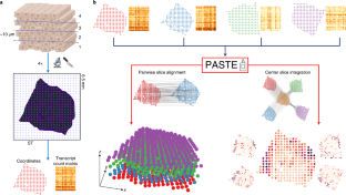
Benchmarking spatial clustering methods with spatially resolved transcriptomics data

A comprehensive benchmarking with practical guidelines for cellular deconvolution of spatial transcriptomics

ClusterMap for multi-scale clustering analysis of spatial gene expression

Data availability.

The ST datasets for the breast cancer 1 , SCC 7 , spinal cord 36 , Her2 breast cancer 37 and DLPFC 12 were taken from the original publications. Preprocessed datasets to reproduce the results can be found at https://doi.org/10.5281/zenodo.6334774 .

Code availability

The PASTE methods are implemented in an open-source, publicly available Python package that is available at https://github.com/raphael-group/paste . All the code to reproduce the analysis can be found at https://github.com/raphael-group/paste_reproducibility .

Ståhl, P. L. et al. Visualization and analysis of gene expression in tissue sections by spatial transcriptomics. Science 353 , 78–82 (2016).

Article PubMed CAS Google Scholar

10x Genomics. Visium spatial gene expression: map the whole transcriptome within the tissue context. https://www.10xgenomics.com/products/spatial-gene-expression/ (accessed October 2020) (2019).

Zhao, E. et al. Spatial transcriptomics at subspot resolution with bayesspace. Nat. Biotechnol. 39 , 1375–1384 (2021).

Article CAS PubMed PubMed Central Google Scholar

Berglund, E. et al. Spatial maps of prostate cancer transcriptomes reveal an unexplored landscape of heterogeneity. Nat. Commun. 9 , 2419 (2018).

Article PubMed PubMed Central CAS Google Scholar

Thrane, K., Eriksson, H., Maaskola, J., Hansson, J. & Lundeberg, J. Spatially resolved transcriptomics enables dissection of genetic heterogeneity in stage iii cutaneous malignant melanoma. Cancer Res. 78 , 5970–5979 (2018).

CAS PubMed Google Scholar

Moncada, R. et al. Integrating microarray-based spatial transcriptomics and single-cell RNA-seq reveals tissue architecture in pancreatic ductal adenocarcinomas. Nat. Biotechnol. 38 , 333–342 (2020).

Article CAS PubMed Google Scholar

Ji, A. et al. Multimodal analysis of composition and spatial architecture in human squamous cell carcinoma. Cell 182 , 1661–1662 (2020).

Chen, W.-T. et al. Spatial transcriptomics and in situ sequencing to study Alzheimer’s disease. Cell 182 , 976–991.e19 (2020).

PubMed Google Scholar

Lundmark, A. et al. Gene expression profiling of periodontitis-affected gingival tissue by spatial transcriptomics. Sci. Rep . 8 , 9370 (2018).

Asp, M. et al. Spatial detection of fetal marker genes expressed at low level in adult human heart tissue. Sci. Rep. 7 , 12941 (2017).

Maniatis, S. et al. Spatiotemporal dynamics of molecular pathology in amyotrophic lateral sclerosis. Science 364 , 89–93 (2019).

Maynard, K. R. et al. Transcriptome-scale spatial gene expression in the human dorsolateral prefrontal cortex. Nat. Neurosci. 24 , 425–436 (2021).

Liu, R. et al. Modeling spatial correlation of transcripts with application to developing pancreas. Sci. Rep . 9 , 5592 (2019).

Svensson, V., Teichmann, S. A. & Stegle, O. SpatialDE: identification of spatially variable genes. Nat. Meth. 15 , 343 (2018).

Article CAS Google Scholar

Arnol, D., Schapiro, D., Bodenmiller, B., Saez-Rodriguez, J. & Stegle, O. Modeling cell-cell interactions from spatial molecular data with spatial variance component analysis. Cell Rep. 29 , 202–211 (2019).

Cang, Z. & Nie, Q. Inferring spatial and signaling relationships between cells from single cell transcriptomic data. Nat. Commun. 11 , 2084 (2020).

Ji, N. & Oudenaarden, A. Single-molecule fluorescent in situ hybridization (smFISH) of C. elegans worms and embryos. In WormBook: The Online Review of C. elegans Biology (ed. WormBook) 1–16 (The C. elegans Research Community, 2012).

Eng, C.-H. L. et al. Transcriptome-scale super-resolved imaging in tissues by RNA seqFISH+. Nature 568 , 235–239 (2019).

Wang, X. et al. Three-dimensional intact-tissue sequencing of single-cell transcriptional states. Science 361 , eaat5691 (2018).

Stickels, R. R. et al. Highly sensitive spatial transcriptomics at near-cellular resolution with slide-seqv2. Nat. Biotechnol. 39 , 313–319 (2021).

Elosua-Bayes, M., Nieto, P., Mereu, E., Gut, I. & Heyn, H. SPOTlight: seeded NMF regression to deconvolute spatial transcriptomics spots with single-cell transcriptomes. Nucleic Acids Res. 49 , e50–e50 (2021).

Bergenstråhle, J., Larsson, L. & Lundeberg, J. Seamless integration of image and molecular analysis for spatial transcriptomics workflows. BMC Genomics 21 , 482 (2020).

Äijö, T. et al. Splotch: robust estimation of aligned spatial temporal gene expression data. Preprint at bioRxiv https://doi.org/10.1101/757096 (2019).

Haghverdi, L., Lun, A. T., Morgan, M. D. & Marioni, J. C. Batch effects in single-cell RNA-sequencing data are corrected by matching mutual nearest neighbors. Nat. Biotechnol. 36 , 421–427 (2018).

Stuart, T. et al. Comprehensive integration of single-cell data. Cell 177 , 1888–1902.e21 (2019).

Hie, B., Bryson, B. & Berger, B. Efficient integration of heterogeneous single-cell transcriptomes using scanorama. Nat. Biotechnol. 37 , 685–691 (2019).

Mandric, I., Hill, B. L., Freund, M. K., Thompson, M. & Halperin, E. Batman: fast and accurate integration of single-cell RNA-seq datasets via minimum-weight matching. iScience 23 , 101185 (2020).

Demetci, P., Santorella, R., Sandstede, B., Noble, W. S. & Singh, R. Gromov-Wasserstein optimal transport to align single-cell multi-omics data. Preprint at bioRxiv https://doi.org/10.1101/2020.04.28.066787 (2020).

Tran, H. T. N. et al. A benchmark of batch-effect correction methods for single-cell RNA sequencing data. Genome Biol. 21 , 12 (2020).

Titouan, V., Courty, N., Tavenard, R. & Flamary, R. Optimal transport for structured data with application on graphs. In International Conference on Machine Learning (eds Chaudhuri, K. & Salakhutdinov, R.) 6275–6284 (PMLR, 2019).

Lee, D. & Seung, H. Algorithms for non-negative matrix factorization. In Advances in Neural Information Processing Systems 13: Proceedings of the 2000 Conference, NIPS 2000 (Neural Information Processing Systems Foundation, 2001).

Shao, C. & Höfer, T. Robust classification of single-cell transcriptome data by nonnegative matrix factorization. Bioinformatics 33 , 235–242 (2016).

Zhu, X., Ching, T., Pan, X., Weissman, S. M. & Garmire, L. Detecting heterogeneity in single-cell RNA-seq data by non-negative matrix factorization. PeerJ 5 , e2888 (2017).

Elyanow, R. et al. STARCH: copy number and clone inference from spatial transcriptomics data. Phys. Biol. 18 , 035001 (2021).

O’Neill, R. et al. Indices of landscape pattern. Landsc. Ecol. 1 , 153–162 (1988).

Article Google Scholar

Andersson, A. et al. Spatial deconvolution of her2 -positive breast cancer delineates tumor-associated cell type interactions. Nat. Commun. 12 , 6012 (2021).

Biancalani, T. et al. Deep learning and alignment of spatially resolved single-cell transcriptomes with Tangram. Nat. Methods 18 , 1352–1362 (2021).

Yoosuf, N., Navarro, J., Salmén, F., Ståhl, P. L. & Daub, C. O. Identification and transfer of spatial transcriptomics signatures for cancer diagnosis. Breast Cancer Res. 22 , 6 (2020).

Brown, L. G. A survey of image registration techniques. ACM Comput. Surv. 24 , 325–376 (1992).

Fatras, K., Zine, Y., Flamary, R., Gribonval, R. & Courty, N. Learning with minibatch Wasserstein: asymptotic and gradient properties. In AISTATS , 2131–2141 http://proceedings.mlr.press/v108/fatras20a.html (2020).

Feydy, J. et al. Interpolating between optimal transport and mmd using sinkhorn divergences. In The 22nd International Conference on Artificial Intelligence and Statistics , 2681–2690 (2019).

Marx, V. Method of the year: spatially resolved transcriptomics. Nat. Methods 18 , 9–14 (2021).

Larsson, L., Frisén, J. & Lundeberg, J. Spatially resolved transcriptomics adds a new dimension to genomics. Nat. Methods 18 , 15–18 (2021).

Wahba, G. A least squares estimate of satellite attitude. SIAM Rev. 7 , 409–409 (1965).

Kabsch, W. A solution for the best rotation to relate two sets of vectors. Acta Crystallogr. A 32 , 922–923 (1976).

Lin, P., Troup, M. & Ho, J. W. K. Cidr: Ultrafast and accurate clustering through imputation for single-cell RNA-seq data. Genome Biology 18 , 59 (2017).

Mongia, A., Sengupta, D. & Majumdar, A. Mcimpute: matrix completion based imputation for single cell RNA-seq data. Frontiers in Genetics 10 , 9 (2019).

Hou, W., Ji, Z., Ji, H. & Hicks, S. C. A systematic evaluation of single-cell RNA-sequencing imputation methods. Genome Biology 21 , 218 (2020).

Févotte, C. & Cemgil, A. T. Nonnegative matrix factorizations as probabilistic inference in composite models. In 2009 17th European Signal Processing Conference , 1913–1917 (IEEE, 2009).

Durif, G., Modolo, L., Mold, J. E., Lambert-Lacroix, S. & Picard, F. Probabilistic count matrix factorization for single cell expression data analysis. Bioinformatics 35 , 4011–4019 (2019).

Townes, F. W., Hicks, S. C., Aryee, M. J. & Irizarry, R. A. Feature selection and dimension reduction for single-cell RNA-seq based on a multinomial model. Genome Biol. 20 , 295 (2019).

Elyanow, R., Dumitrascu, B., Engelhardt, B. E. & Raphael, B. J. netnmf-sc: leveraging gene-gene interactions for imputation and dimensionality reduction in single-cell expression analysis. Genome Res. 30 , 195–204 (2020).

Wolf, F. A., Angerer, P. & Theis, F. J. Scanpy: large-scale single-cell gene expression data analysis. Genome Biology 19 , 15 (2018).

Article PubMed PubMed Central Google Scholar

Flamary, R. & Courty, N. Pot Python Optimal Transport Library https://pythonot.github.io/ (2017).

Sun, S., Zhu, J., Ma, Y. & Zhou, X. Accuracy, robustness and scalability of dimensionality reduction methods for single-cell RNA-seq analysis. Genome Biol. 20 , 269 (2019).

Chen, M. & Zhou, X. Viper: variability-preserving imputation for accurate gene expression recovery in single-cell RNA sequencing studies. Genome Biol. 19 , 196 (2018).

Download references

Acknowledgements

This work was supported by National Cancer Institute grants U24CA211000 and U24CA248453 to B.J.R. The funder had no role in the conceptualization, design, data collection, analysis, decision to publish or preparation of the manuscript.

Author information

Authors and affiliations.

Department of Computer Science, Princeton University, Princeton, NJ, USA

Ron Zeira, Max Land, Alexander Strzalkowski & Benjamin J. Raphael

You can also search for this author in PubMed Google Scholar

Contributions

R.Z. conceived, designed and developed the method, analyzed the DLPFC and Her2 breast cancer datasets and wrote the manuscript with contributions from the coauthors. M.L. implemented the method and performed the simulation, SCC and spinal cord data analyses. A.S. contributed to the benchmarking of PASTE against Seurat and STUtility and the analyses of the DLPFC and SCC dataset. B.J.R. supervised the work, contributed to the design of the method and wrote the manuscript with contributions from the coauthors. All authors read and approved the final manuscript.

Corresponding author

Correspondence to Benjamin J. Raphael .

Ethics declarations

Competing interests.

B.J.R. is a cofounder of, and consultant to, Medley Genomics. The other authors declare no competing interests.

Peer review

Peer review information.

Nature Methods thanks Jean Yang and the other, anonymous, reviewers for their contribution to the peer review of this work. Lei Tang was the primary editor on this article and managed its editorial process and peer review in collaboration with the rest of the editorial team.

Additional information

Publisher’s note Springer Nature remains neutral with regard to jurisdictional claims in published maps and institutional affiliations.

Extended data

Extended data fig. 1 spatial organization of breast cancer st slices..

(a-d) Spatial organization of the four breast cancer ST slices from 35 . Each slice in this dataset consists of 251-264 spots and 7453-7998 genes. (e) Spatial coordinates of the four breast cancer ST slices from 35 after pairwise alignment via PASTE.

Extended Data Fig. 2 PASTE results on simulated data generated from each of the indicated breast cancer slices 35 .

Each line (color) corresponds to running PASTE with a specific value for alpha. Error bars represent the standard deviation across 10 simulated instances.

Extended Data Fig. 3 Comparison of published clusters and clusters obtained by PASTE on ST data from SCC patients 2, 5, 9, and 10 in 21 .

(Left) The published cluster labels from 21 of spots in slice A from each of the four patients. (Right) k -means clustering of inferred center slice from PASTE.

Extended Data Fig. 4 PASTE integration of Her2 breast cancer patient G from Andersson et al.

(a) Pathological annotations and (b) clustering results from PASTE integrated slice for a slice of breast cancer patient G from Andersson et al. Black circles indicate small region of spots of in situ cancer which are also clustered together in the PASTE integrated slice.

Extended Data Fig. 5 Dorsolateral prefrontal cortex ST data from 31 .

Each of the three samples is composed of four ST slices. The first two slices and last two slices are 10 μ m apart while the middle pair of slices is taken 300 μ m apart. Spots are colored by the six neocortical layers or the white matter according to the annotation of 31 .

Extended Data Fig. 6 Pairwise alignment of slices B and C from DLPFC Sample I.

Pairwise alignment using (a) PASTE, (b) Seurat, (c) Tangram and (d) STUtility. Gray lines connect the 1000 spot pairs with highest alignment values from each method. PASTE and STUtility alignments are more consistent with spatial organization of slices than Seurat and Tangram alignments.

Extended Data Fig. 7 Alignment accuracy of adjacent DLPFC slices using PASTE with different expression costs.

PASTE with: (Default) All genes and KL divergence, (Lib-Log-Norm) All genes with library size normalization and log transformation and Euclidean distance, (HVG) Same as Lib-Log-Norm but restricted to top 2000 highly variable genes.

Extended Data Fig. 8 TRABD2A expression in a single slice and PASTE integrated slice.

The boundaries between the layers are marked in green in a and c. WM and Layers 6 to 1 have 625, 614, 621, 247, 924, 224 and 380 spots respectively. Inner boxplots show the 25%, 50% and 75% quantiles of the distributions. p -values (rounded to the closest power of 10) for the difference in distribution (two-sided Mann-Whitney U test) between adjacent layers are indicated. TRABD2A was validated using smFISH in 31 as a layer 5 marker gene.

Extended Data Fig. 9 Ranking of known layer-specific marker genes by differential expression analysis.

Gene ranking using: the pseudo-bulk approach of Maynard et al., PASTE center slice integration, Scanorama, and Seurat. Red lines indicate median rank of marker genes which are 1147 for Maynard et al, 427 for PASTE, 3380.5 for Scanorama, and 1852 for Seurat. Rank 1 is the highest rank.

Supplementary information

Supplementary information, reporting summary, peer review file, rights and permissions.

Reprints and permissions

About this article

Cite this article.

Zeira, R., Land, M., Strzalkowski, A. et al. Alignment and integration of spatial transcriptomics data. Nat Methods 19 , 567–575 (2022). https://doi.org/10.1038/s41592-022-01459-6

Download citation

Received : 16 July 2021

Accepted : 17 March 2022

Published : 16 May 2022

Issue Date : May 2022

DOI : https://doi.org/10.1038/s41592-022-01459-6

Share this article

Anyone you share the following link with will be able to read this content:

Sorry, a shareable link is not currently available for this article.

Provided by the Springer Nature SharedIt content-sharing initiative

This article is cited by

Mnmst: topology of cell networks leverages identification of spatial domains from spatial transcriptomics data.

Genome Biology (2024)

Multi-slice spatial transcriptome domain analysis with SpaDo

Shaoqi Chen

SANTO: a coarse-to-fine alignment and stitching method for spatial omics

Yingxin Lin

Nature Communications (2024)

Cross-modality mapping using image varifolds to align tissue-scale atlases to molecular-scale measures with application to 2D brain sections

Kaitlin M. Stouffer
Alain Trouvé
Michael I. Miller

Simulating multiple variability in spatially resolved transcriptomics with scCube

Jingyang Qian

Quick links

Explore articles by subject
Guide to authors
Editorial policies

IMAGES

Cell clustering for spatial transcriptomics data with graph neural
C-SIDE learns cell type-specific DE from spatial transcriptomics
Spatial Transcriptomics
ClusterMap across different spatial transcriptomics methods a Cell type
(PDF) Multiscale topology classifies and quantifies cell types in
Cell type calling of spatial transcriptomics data using FR-Match. (A

VIDEO

8 Visium data: Subset and integrate with single-cell data (update, August 2023)
Short Talks: Spatial Transcriptomics
Spatial Data Analysis Using Giotto: 3D MERfish Dataset Analysis Part II
Spatial Data Analysis Using Giotto: CODEX (Akoya PhenoCycler) Mouse Spleen Dataset
Corrplot Video Tutorial 1: Method, Order, Type & Diag
scRNA-seq Data Analysis Using Giotto, Part II: Differential Expression and Cell Type Annotation

COMMENTS

Cell Type Assignments for Spatial Transcriptomics Data
A key question in the initial analysis of such spatial transcriptomics data is the assignment of cell types. To date, most studies used methods that only rely on the expression levels of the genes in each cell for such assignments. To fully utilize the data and to improve the ability to identify novel sub-types we developed a new method, FICT ...
Probabilistic cell/domain-type assignment of spatial transcriptomics
To address the challenges presented by spatial annotation, we propose the use of a probabilistic model, SpatialAnno, which performs cell/domain-type assignments for SRT data and has the capability of leveraging non-marker genes to assign cell/domain types via a factor model while accounting for spatial information via a Potts model (16, 17). To ...
Probabilistic cell/domain-type assignment of spatial transcriptomics
Abstract. In the analysis of both single-cell RNA sequencing (scRNA-seq) and spatially resolved transcriptomics (SRT) data, classifying cells/spots into cell/domain types is an essential analytic step for many secondary analyses. Most of the existing annotation methods have been developed for scRNA-seq datasets without any consideration of ...
Cell Type Assignments for Spatial Transcriptomics Data
A key question in the initial analysis of such spatial transcriptomics data is the assignment of cell types. To date, most studies used methods that only rely on the expression levels of the genes in each cell for such assignments. To fully utilize the data and to improve the ability to identify novel sub-types we developed a new method, FICT ...
Spatial-ID: a cell typing method for spatially resolved transcriptomics
Comprehensive annotating of cell types in spatially resolved transcriptomics to understand biological processes at the single cell level remains challenging. Here the authors introduce Spatial-ID ...
Mapping cellular interactions from spatially resolved transcriptomics data
Spacia is a multiple-instance learning model for cell-cell communication (CCC) interference in single-cell resolution spatially resolved transcriptomics data. Spacia can map complex CCCs by ...
Intracellular spatial transcriptomic analysis toolkit (InSTAnT)
The dataset contained 6325 cells with 553 average number of transcripts across 7 z-planes. We obtained cell type assignment from Supplememtary Data 1 from Moffit et al. 54. We removed ambiguous ...
ScType enables fast and accurate cell type identification from spatial
For instance, if a spot was labeled as "Immune cell" by the pathologist, cell type assignments of "T cell," "Dendritic cell," or "B cell" would all be ... we repurposed the existing scType tool to annotate cell types from spatial transcriptomics data and benchmarked its performance against existing spatial cell type annotation ...
Cell-type modeling in spatial transcriptomics data elucidates spatially
Since scRNA-seq profiles the transcriptome, including the marker genes, we can assign cell-types unambiguously to the cells in scRNA-seq data. Using these cell-type assignments in the scRNA-seq data, we can build models that learn to map a cell to its cell-type, i.e., classify the cell, given the transcriptional expression of only the shared ...
Cell Type Assignments for Spatial Transcriptomics Data
the initial analysis of such spatial transcriptomics data is the assignment of cell t ypes. To date, most. studies used methods that only rely on the expression levels of the genes in each cell ...
PDF Cell-type modeling in spatial transcriptomics data ...
Cell-type modeling in spatial transcriptomics data elucidates spatially variable colocalization and communication between cell-types in mouse brain Francisco Jose Grisanti Canozo,1,2 Zhen Zuo,1 James F. Martin,1,2 and Md. Abul Hassan Samee1,3,* 1Baylor College of Medicine, Houston, TX 77030, USA 2Texas Heart Institute, Houston, TX 77030, USA ...
Cell-type modeling in spatial transcriptomics data elucidates spatially
We developed a neural network model, spatial transcriptomics cell-types assignment using neural networks (STANN), to overcome these challenges. Analysis of STANN's predicted cell types in mouse olfactory bulb (MOB) sc-ST data delineated MOB architecture beyond its morphological layer-based conventional description. We find that cell-type ...
Mapping the transcriptome: Realizing the full potential of spatial data
Modern spatial transcriptomics methods generate three distinct but interrelated data types: (1) the image data, (2) the expression data, and (3) the spatial orientation and location of (2). A typical spatial transcriptomics analysis workflow (e.g., Orchestrating Spatially-Resolved Transcriptomics Analysis with Bioconductor) tends to treat ...
Cell-type modeling in spatial transcriptomics data ...
Grisanti Canozo et al. developed a neural network, STANN, to model cell types in single-cell-resolution spatial transcriptomics (sc-ST) data. They deployed STANN within a pipeline for careful feature selection and class imbalance-aware model fitting. STANN's predicted cell types in mouse olfactory bulb (MOB) sc-ST data revealed high spatial variations in cellular colocalization and ...
Mapping cellular interactions from spatially resolved transcriptomics data
Cell-cell communication (CCC) is essential to how life forms and functions. However, accurate, high-throughput mapping of how expression of all genes in one cell affects expression of all genes in another cell is made possible only recently through the introduction of spatially resolved transcriptomics (SRT) technologies, especially those that achieve single-cell resolution.
Reference-based cell type matching of in situ image-based spatial
In parallel, spot-based cell type assignment was performed by SSAM 32 using a guided mode, which partially borrows information from the combined assignment results. All spatial data and cell type ...
ST-SCSR: identifying spatial domains in spatial transcriptomics data
However, scRNA-seq lose spatial coordination of cells, failing to fully characterize micro-environments of tissue. Fortunately, recent advances in spatial transcriptomics (ST) enable the simultaneous measurement of expression profile and spatial information of cells, offering a new perspective to model the complicated structure of tissues .
Single-cell and spatial transcriptomics enables probabilistic inference
The framework we propose uses single-cell data to infer proportion estimates of each cell type at every capture location within the spatial data, eliminating any need for interpretation or ...
PDF Probabilistic cell/domain-type assignment of spatial transcriptomics
Uniquely, SpatialAnno, via the factor model, allows for the assignment of cell/ domain types that leverage a large number of non-marker genes, and, via the Potts model, is more likely to assign ...
A comprehensive comparison on cell-type composition inference for
Realizing the critical importance of cell-type decomposition, multiple groups have developed ST deconvolution methods. The aim of this work is to review state-of-the-art methods for ST deconvolution, comparing their strengths and weaknesses. In particular, we construct ST spots from single-cell level ST data to assess the performance of 10 ...
A standard for sharing spatial transcriptomics data
Spatial transcriptomic technologies have the potential to reveal critical relationships between the function of genes and cells and their spatial organization. Here, we provide a sharing model for spatial transcriptomics data with the aim of establishing a set of primary data and metadata needed to reproduce analyses and facilitate computational methods development.
Probabilistic cell/domain-type assignment of spatial transcriptomics
SpatialAnno is presented, an efficient and accurate annotation method for spatial transcriptomics datasets, with the capability to effectively leverage a large number of non-marker genes as well as "qualitative" information about marker genes without using a reference dataset. In the analysis of both single-cell RNA sequencing (scRNA-seq) and spatially resolved transcriptomics (SRT) data ...
Unraveling the spatial organization and development of human ...
CellPhoneDB 32 (version v5.0), a repository of ligand-receptor interactions, was employed to identify enriched interactions between various cell types in single-cell transcriptomics data. To ...
CHAI: consensus clustering through similarity matrix integration for
We represent a cell to clustering assignment vector as a binary similarity matrix using the following rules: (i) If two cells have the same clustering assignment, assign a value of 1 to a binary similarity matrix corresponding to the two cells. ... Stgnnks: identifying cell types in spatial transcriptomics data based on graph neural network ...
IJMS
Limb muscle is responsible for physical activities and myogenic cell migration during embryogenesis is indispensable for limb muscle formation. Maternal obesity (MO) impairs prenatal skeletal muscle development, but the effects of MO on myogenic cell migration remain to be examined. C57BL/6 mice embryos were collected at E13.5. The GeoMx DSP platform was used to customize five regions along ...
Probabilistic cell/domain-type assignment of spatial transcriptomics
In the analysis of both single-cell RNA sequencing (scRNA-seq) and spatially resolved transcriptomics (SRT) data, classifying cells/spots into cell/domain types is an essential analytic step for many secondary analyses. Most of the existing annotation methods have been developed for scRNA-seq datasets without any consideration of spatial information. Here, we present SpatialAnno, an efficient ...
Probabilistic cell/domain-type assignment of spatial transcriptomics
In the analysis of both single-cell RNA sequencing (scRNA-seq) and spatially resolved transcriptomics (SRT) data, classifying cells/spots into cell/domain types is an essential analytic step for many secondary analyses. Most of the existing annotation methods have been developed for scRNA-seq datasets without any consideration of spatial ...
Cell-type modeling in spatial transcriptomics data elucidates spatially
Since scRNA-seq profiles the transcriptome, including the marker genes, we can assign cell types unambiguously to the cells in scRNA-seq data. Using these cell-type assignments in the scRNA-seq data, we can build models that learn to map a cell to its cell type, i.e., classify the cell, given the transcriptional expression of only the shared ...
Integrating spatial and single-cell transcriptomics data using deep
Spatial transcriptomics (ST) is transforming tissue analysis but has limitations. Here, authors introduce SpatialScope, an integrated approach combining scRNA-seq and ST data using deep generative ...
Alignment and integration of spatial transcriptomics data
Alignment and integration of spatial transcriptomics data

Save citation to file

Add to My Bibliography

A comprehensive comparison on cell-type composition inference for spatial transcriptomics data

Similar articles

Publication types

Grants and funding

LinkOut - more resources

Probabilistic cell/domain-type assignment of spatial transcriptomics data with SpatialAnno

63 References

Joint dimension reduction and clustering analysis of single-cell RNA-seq and spatial transcriptomics data

Article Contents

CHAI: consensus clustering through similarity matrix integration for cell-type identification

Individual clustering algorithms

CHAI-AvgSim

GraphST binary matrix representation for spatial transcriptomics

Evaluation metrics

Normalized mutual information

Silhouette score

CHAI workflow

CHAI outperforms existing clustering methods on benchmarking datasets

CHAI outperforms existing clustering methods across varying dataset sizes and complexity

CHAI derives validated biological insights in a breast cancer dataset: case study

Integration of spatial transcriptomics data with CHAI: CHAI-ST

Baron pancreas data

Muraro pancreas data

SC-Mixology data

Zeisel mouse brain

Zheng 68K PBMC data

Savas breast cancer T Cell Data

Vandenbon mouse liver cancer visium data

Supplementary data

Email alerts

Affiliations

This Feature Is Available To Subscribers Only

Information

Initiatives

Article Menu

JSmol Viewer

1. Introduction

Share and Cite

Article Metrics

Probabilistic cell/domain-type assignment of spatial transcriptomics data with SpatialAnno

Competing Interest Statement

Citation Manager Formats

Subject Area

Probabilistic cell/domain-type assignment of spatial transcriptomics data with SpatialAnno

Zhenxing Guo

Chaolong Wang

Associated Data

Graphical Abstract

Introduction

Materials and methods

Methods for comparison

Simulations

Real datasets

Mouse olfactory bulb data by spatial transcriptomics (ST)

Mouse hippocampus Slide-seq data and Slide-seqV2 data

Mouse embryo data by seqFISH

Evaluation metrics

Overview of SpatialAnno

Validation using simulated data

SpatialAnno improves annotations of known layers in human dorsolateral prefrontal cortex

SpatialAnno correctly identifies cells in mouse olfactory bulb

SpatialAnno reveals cell-type distribution in mouse hippocampus with SRT data at near-cell resolution

Embeddings estimated by SpatialAnno lead to biologically relevant trajectories in mouse embryo

Supplementary Material

Contributor Information

Data availability

Alignment and integration of spatial transcriptomics data

Access options

Similar content being viewed by others

Benchmarking spatial clustering methods with spatially resolved transcriptomics data

A comprehensive benchmarking with practical guidelines for cellular deconvolution of spatial transcriptomics

ClusterMap for multi-scale clustering analysis of spatial gene expression

Code availability

Acknowledgements

Author information

Contributions

Corresponding author

Ethics declarations