Instantly share code, notes, and snippets.

rooneyroy / gist:f34276fa3049a598d2401ef64189133b
- Download ZIP
- Star ( 0 ) 0 You must be signed in to star a gist
- Fork ( 0 ) 0 You must be signed in to fork a gist
- Embed Embed this gist in your website.
- Share Copy sharable link for this gist.
- Clone via HTTPS Clone using the web URL.
- Learn more about clone URLs
- Save rooneyroy/f34276fa3049a598d2401ef64189133b to your computer and use it in GitHub Desktop.
| # Set Working Directory | |
| setwd("F:/IIITB - Upgrad/Course 3 - Predictive Analysis/Case Study") | |
| # Install and Load the required packages | |
| install.packages("MASS") | |
| install.packages("car") | |
| install.packages("e1071") | |
| install.packages("ROCR") | |
| install.packages("caret") | |
| install.packages("Hmisc") | |
| install.packages("plyr") | |
| install.packages("ggplot2") | |
| install.packages("moments") | |
| install.packages("arules") | |
| install.packages("ROCR") | |
| install.packages("class") | |
| library(ROCR) | |
| library(arules) | |
| library(MASS) | |
| library(car) | |
| library(caret) | |
| library(ROCR) | |
| library(e1071) | |
| library(Hmisc) | |
| library(plyr) | |
| library(ggplot2) | |
| library(arules) | |
| library(class) | |
| #Checkpoint 1 | |
| # Load the given files. | |
| churn_data <- read.csv("churn_data.csv", stringsAsFactors = FALSE) | |
| customer_data <- | |
| read.csv("customer_data.csv", stringsAsFactors = FALSE) | |
| internet_data <- | |
| read.csv("internet_data.csv", stringsAsFactors = FALSE) | |
| str(churn_data) | |
| str(customer_data) | |
| str(internet_data) | |
| # Collate the 3 files in a single file. | |
| merge1 <- merge(churn_data, customer_data, by = 'customerID') | |
| churn <- merge(merge1, internet_data, by = 'customerID') | |
| # Understand the structure of the collated file. | |
| str(churn) | |
| #Checkpoint 2 - EDA | |
| # Make bar charts to find interesting relationships between variables. | |
| #Distribution of monthly charges along with churn | |
| ggplot(churn, aes(x = churn$MonthlyCharges)) + geom_histogram() + aes(fill = churn$Churn) | |
| #Distribution of tenure along with churn | |
| ggplot(churn, aes(x = churn$tenure)) + geom_histogram() + aes(fill = churn$Churn) | |
| #Gender wise churn | |
| ggplot(churn, aes(x = churn$Churn, fill = churn$gender)) + geom_bar() | |
| #internet service wise churn | |
| ggplot(churn, aes(x = churn$InternetService, fill = churn$Churn)) + geom_bar() | |
| #payment method wise churn | |
| ggplot(churn, aes(x = churn$PaymentMethod, fill = churn$Churn)) + geom_bar() | |
| #Techsupport wise churn | |
| ggplot(churn, aes(x = churn$TechSupport, fill = churn$Churn)) + geom_bar() | |
| #Checkpoint 3 - Data Preparation | |
| # Make Box plots for numeric variables to look for outliers. | |
| boxplot(churn$tenure) | |
| boxplot.stats(churn$tenure) #No Outlier | |
| boxplot(churn$MonthlyCharges) | |
| boxplot.stats(churn$MonthlyCharges) #No Outlier | |
| boxplot(churn$TotalCharges) | |
| boxplot.stats(churn$TotalCharges) #No Outlier | |
| # Perform De-Duplication if required | |
| which(duplicated(churn) == 'TRUE') #No Duplicates | |
| # Impute the missing values, and perform the outlier treatment. | |
| sapply(churn, function(x) | |
| sum(is.na(x))) | |
| churn$TotalCharges[which(is.na(churn$TotalCharges) == 'TRUE')] <- | |
| mean(churn$TotalCharges, na.rm = TRUE) | |
| #CHECKPOINT 4: Modeling | |
| #Model 1: Logistics Regression | |
| #Creating object for modeling | |
| churn_df = cbind.data.frame(churn$tenure, churn$MonthlyCharges, churn$TotalCharges) | |
| names(churn_df)[names(churn_df) == 'churn$tenure'] <- 'tenure' | |
| names(churn_df)[names(churn_df) == 'churn$MonthlyCharges'] <- | |
| 'MonthlyCharges' | |
| names(churn_df)[names(churn_df) == 'churn$TotalCharges'] <- | |
| 'TotalCharges' | |
| # Bring the variables in the correct format | |
| dummy_PhoneService = as.data.frame(model.matrix( ~ PhoneService - 1, data = churn)) | |
| churn_df = cbind(churn_df, dummy_PhoneService[, -1]) | |
| names(churn_df)[names(churn_df) == 'dummy_PhoneService[, -1]'] <- | |
| 'dummy_PhoneService' | |
| dummy_PaperlessBilling = as.data.frame(model.matrix( ~ PaperlessBilling - | |
| 1, data = churn)) | |
| churn_df = cbind(churn_df, dummy_PaperlessBilling[, -1]) | |
| names(churn_df)[names(churn_df) == 'dummy_PaperlessBilling[, -1]'] <- | |
| 'dummy_PaperlessBilling' | |
| dummy_Churn = as.data.frame(model.matrix( ~ Churn - 1, data = churn)) | |
| churn_df = cbind(churn_df, dummy_Churn[, -1]) | |
| names(churn_df)[names(churn_df) == 'dummy_Churn[, -1]'] <- | |
| 'dummy_Churn' | |
| dummy_gender = as.data.frame(model.matrix( ~ gender - 1, data = churn)) | |
| churn_df = cbind(churn_df, dummy_gender[, -1]) | |
| names(churn_df)[names(churn_df) == 'dummy_gender[, -1]'] <- | |
| 'dummy_gender' | |
| #Senior Citizen data is already in 0-1 format, changing it to numeric | |
| churn_df = cbind(churn_df, as.numeric(churn$SeniorCitizen)) | |
| names(churn_df)[names(churn_df) == 'as.numeric(churn$SeniorCitizen)'] <- | |
| 'dummy_SeniorCitizen' | |
| dummy_Partner = as.data.frame(model.matrix( ~ Partner - 1, data = churn)) | |
| churn_df = cbind(churn_df, dummy_Partner[, -1]) | |
| names(churn_df)[names(churn_df) == 'dummy_Partner[, -1]'] <- | |
| 'dummy_Partner' | |
| dummy_Dependents = as.data.frame(model.matrix( ~ Dependents - 1, data = churn)) | |
| churn_df = cbind(churn_df, dummy_Dependents[, -1]) | |
| names(churn_df)[names(churn_df) == 'dummy_Dependents[, -1]'] <- | |
| 'dummy_Dependents' | |
| dummy_contract = as.data.frame(model.matrix( ~ Contract - 1, data = churn)) | |
| churn_df = cbind(churn_df, dummy_contract[, -3]) | |
| dummy_PaymentMethod = as.data.frame(model.matrix( ~ PaymentMethod - 1, data = churn)) | |
| churn_df = cbind(churn_df, dummy_PaymentMethod[, -4]) | |
| dummy_InternetService = as.data.frame(model.matrix( ~ InternetService - | |
| 1, data = churn)) | |
| churn_df = cbind(churn_df, dummy_InternetService[, -3]) | |
| dummy_OnlineSecurity = as.data.frame(model.matrix( ~ OnlineSecurity - 1, data = churn)) | |
| churn_df = cbind(churn_df, dummy_OnlineSecurity[, -3]) | |
| dummy_OnlineBackup = as.data.frame(model.matrix( ~ OnlineBackup - 1, data = churn)) | |
| churn_df = cbind(churn_df, dummy_OnlineBackup[, -3]) | |
| dummy_multiplelines = as.data.frame(model.matrix( ~ MultipleLines - 1, data = churn)) | |
| churn_df = cbind(churn_df, dummy_multiplelines[, -3]) | |
| dummy_DeviceProtection = as.data.frame(model.matrix( ~ DeviceProtection - | |
| 1, data = churn)) | |
| churn_df = cbind(churn_df, dummy_DeviceProtection[, -3]) | |
| dummy_TechSupport = as.data.frame(model.matrix( ~ TechSupport - 1, data = churn)) | |
| churn_df = cbind(churn_df, dummy_TechSupport[, -3]) | |
| dummy_StreamingTV = as.data.frame(model.matrix( ~ StreamingTV - 1, data = churn)) | |
| churn_df = cbind(churn_df, dummy_StreamingTV[, -3]) | |
| dummy_StreamingMovies = as.data.frame(model.matrix( ~ StreamingMovies - | |
| 1, data = churn)) | |
| churn_df = cbind(churn_df, dummy_StreamingMovies[, -3]) | |
| str(churn_df) | |
| #Split data set | |
| set.seed(100) | |
| train.indices = sample(1:nrow(churn_df), 0.7 * nrow(churn_df)) | |
| train.data = churn_df[train.indices,] | |
| test.data = churn_df[-train.indices,] | |
| # Initial Model with all variables | |
| initial_model = glm(dummy_Churn ~ ., data = train.data, family = "binomial") | |
| summary(initial_model) | |
| # Stepwise selection | |
| step_model = step(initial_model, direction = "both") | |
| summary(step_model) | |
| vif(step_model) | |
| dummy_Churn ~ tenure + MonthlyCharges + TotalCharges + dummy_PhoneService + | |
| dummy_PaperlessBilling + dummy_SeniorCitizen + `ContractMonth-to-month` + `ContractOne year` + | |
| `PaymentMethodElectronic check` + InternetServiceDSL + OnlineSecurityNo + | |
| OnlineBackupNo + TechSupportNo | |
| #Remove Tenure (High VIF) | |
| model1 = glm( | |
| dummy_Churn ~ MonthlyCharges + TotalCharges + dummy_PhoneService + | |
| dummy_PaperlessBilling + dummy_SeniorCitizen + `ContractMonth-to-month` + `ContractOne year` + | |
| `PaymentMethodElectronic check` + InternetServiceDSL + OnlineSecurityNo + | |
| OnlineBackupNo + TechSupportNo, | |
| data = train.data, | |
| family = "binomial" | |
| ) | |
| summary(model1) | |
| vif(model1) | |
| #Remove ContractMonth-to-month (High VIF) | |
| model2 = glm( | |
| dummy_Churn ~ MonthlyCharges + TotalCharges + dummy_PhoneService + | |
| dummy_PaperlessBilling + dummy_SeniorCitizen + `ContractOne year` + | |
| `PaymentMethodElectronic check` + InternetServiceDSL + OnlineSecurityNo + | |
| OnlineBackupNo + TechSupportNo, | |
| data = train.data, | |
| family = "binomial" | |
| ) | |
| summary(model2) | |
| vif(model2) | |
| #Remove OnlineBackupNo (Insignificant) | |
| model3 = glm( | |
| dummy_Churn ~ MonthlyCharges + TotalCharges + dummy_PhoneService + | |
| dummy_PaperlessBilling + dummy_SeniorCitizen + `ContractOne year` + | |
| `PaymentMethodElectronic check` + InternetServiceDSL + OnlineSecurityNo + | |
| TechSupportNo, | |
| data = train.data, | |
| family = "binomial" | |
| ) | |
| summary(model3) | |
| vif(model3) | |
| #Checking correlation between MonthlyCharges & TotalCharges | |
| cor(train.data$MonthlyCharges, train.data$TotalCharges) | |
| #Since strong correlation, removing MonthlyCharges | |
| model4 = glm( | |
| dummy_Churn ~ TotalCharges + dummy_PhoneService + | |
| dummy_PaperlessBilling + dummy_SeniorCitizen + `ContractOne year` + | |
| `PaymentMethodElectronic check` + InternetServiceDSL + OnlineSecurityNo + | |
| TechSupportNo, | |
| data = train.data, | |
| family = "binomial" | |
| ) | |
| summary(model4) | |
| vif(model4) | |
| #Removing dummy_PhoneService (low significance) | |
| model5 = glm( | |
| dummy_Churn ~ TotalCharges + dummy_PaperlessBilling + dummy_SeniorCitizen + `ContractOne year` + | |
| `PaymentMethodElectronic check` + InternetServiceDSL + OnlineSecurityNo + | |
| TechSupportNo, | |
| data = train.data, | |
| family = "binomial" | |
| ) | |
| summary(model5) | |
| vif(model5) | |
| #Removing dummy_SeniorCitizen (low significance) | |
| model6 = glm( | |
| dummy_Churn ~ TotalCharges + dummy_PaperlessBilling + `ContractOne year` + | |
| `PaymentMethodElectronic check` + InternetServiceDSL + OnlineSecurityNo + | |
| TechSupportNo, | |
| data = train.data, | |
| family = "binomial" | |
| ) | |
| summary(model6) | |
| vif(model6) | |
| best_model_log = model6 | |
| summary(best_model_log) | |
| ## C-statistic | |
| train.data$predicted_prob = predict(best_model_log, type = "response") | |
| rcorr.cens(train.data$predicted_prob, train.data$dummy_Churn) | |
| test.data$predicted_prob = predict(best_model_log, newdata = test.data, type = "response") | |
| rcorr.cens(test.data$predicted_prob, test.data$dummy_Churn) | |
| #KS-statistic | |
| #Train Data | |
| model_score <- | |
| prediction(train.data$predicted_prob, train.data$dummy_Churn) | |
| model_perf <- performance(model_score, "tpr", "fpr") | |
| ks_table <- | |
| attr(model_perf, "y.values")[[1]] - (attr(model_perf, "x.values")[[1]]) | |
| ks = max(ks_table) | |
| ks | |
| which(ks_table == ks) | |
| #Test Data | |
| model_score_test <- | |
| prediction(test.data$predicted_prob, test.data$dummy_Churn) | |
| model_perf_test <- performance(model_score_test, "tpr", "fpr") | |
| ks_table_test <- | |
| attr(model_perf_test, "y.values")[[1]] - (attr(model_perf_test, "x.values")[[1]]) | |
| ks_test = max(ks_table_test) | |
| ks_test | |
| which(ks_table_test == ks_test) | |
| # Selecting threshold value | |
| # ROC curve | |
| plot(model_perf, col = "red", lab = c(10, 10, 10)) | |
| plot(model_perf_test, col = "red", lab = c(10, 10, 10)) | |
| #confusion matrix 1 (Threshold Value = 0.5) | |
| confusionMatrix(as.numeric(train.data$predicted_prob > 0.5), | |
| train.data$dummy_Churn, | |
| positive = "1") | |
| confusionMatrix(as.numeric(test.data$predicted_prob > 0.5), | |
| test.data$dummy_Churn, | |
| positive = "1") | |
| #confusion matrix 2 (Threshold Value = 0.3) | |
| confusionMatrix(as.numeric(train.data$predicted_prob > 0.3), | |
| train.data$dummy_Churn, | |
| positive = "1") | |
| confusionMatrix(as.numeric(test.data$predicted_prob > 0.3), | |
| test.data$dummy_Churn, | |
| positive = "1") | |
| #confusion matrix 3 (Threshold Value = 0.7) | |
| confusionMatrix(as.numeric(train.data$predicted_prob > 0.7), | |
| train.data$dummy_Churn, | |
| positive = "1") | |
| confusionMatrix(as.numeric(test.data$predicted_prob > 0.7), | |
| test.data$dummy_Churn, | |
| positive = "1") | |
| # Model2 | |
| # K-NN Model: | |
| #Creating "churn_knn" dataframe from "churn_df" and bringing original churn data | |
| churn_knn = churn_df[, -6] | |
| churn_knn = cbind(churn_knn, as.factor(churn$Churn)) | |
| names(churn_knn)[names(churn_knn) == 'as.factor(churn$Churn)'] <- | |
| 'Churn' | |
| # Bring the data in the correct format to implement K-NN model. | |
| churn_knn$MonthlyCharges <- scale(churn_knn$MonthlyCharges) | |
| churn_knn$TotalCharges <- scale(churn_knn$TotalCharges) | |
| # Implement the K-NN model for optimal K. | |
| set.seed(2) | |
| s1 = sample(1:nrow(churn_knn), 0.7 * nrow(churn_knn)) | |
| churn_knn_train = churn_knn[s1, ] | |
| churn_knn_test = churn_knn[-s1, ] | |
| cl <- churn_knn_train[, 31] | |
| #Removing Class label "dummy_churn" from the train and test data set | |
| churn_knn_train1 <- churn_knn_train[, -31] | |
| churn_knn_test1 <- churn_knn_test[, -31] | |
| #Using the train() command to find the best K. | |
| model <- train( | |
| Churn ~ ., | |
| data = churn_knn_train, | |
| method = 'knn', | |
| tuneGrid = expand.grid(.k = 1:50), | |
| metric = 'Accuracy', | |
| trControl = trainControl( | |
| method = 'repeatedcv', | |
| number = 10, | |
| repeats = 10 | |
| ) | |
| ) | |
| #Generating the plot of the model | |
| model | |
| plot(model) # Looking at graph we can see that optimum K = 19 (Post which not much difference in accuracy) | |
| #Creating the model with optimum cost | |
| impknn2 <- | |
| knn(churn_knn_train1, | |
| churn_knn_test1, | |
| cl, | |
| k = 19, | |
| prob = TRUE) | |
| table(impknn2, churn_knn_test[, 31]) | |
| confusionMatrix(impknn2, churn_knn_test[, 31], positive = "Yes") | |
| #KNN Model Solution | |
| # Accuracy = 79.32% | |
| # Sensitivity = 50.98% | |
| # Specificity = 89.51% | |
| ########################################################################## | |
| # Model 3 | |
| # Naive Bayes Model: | |
| #Using the original data set | |
| str(churn) | |
| # Bring the data in the correct format to implement Naive Bayes algorithm. | |
| churn$customerID <- factor(churn$customerID) | |
| churn$PhoneService <- factor(churn$PhoneService) | |
| churn$Contract <- factor(churn$Contract) | |
| churn$PaperlessBilling <- factor(churn$PaperlessBilling) | |
| churn$PaymentMethod <- factor(churn$PaymentMethod) | |
| churn$Churn <- factor(churn$Churn) | |
| churn$gender <- factor(churn$gender) | |
| churn$Partner <- factor(churn$Partner) | |
| churn$Dependents <- factor(churn$Dependents) | |
| churn$MultipleLines <- factor(churn$MultipleLines) | |
| churn$InternetService <- factor(churn$InternetService) | |
| churn$OnlineSecurity <- factor(churn$OnlineSecurity) | |
| churn$OnlineBackup <- factor(churn$DeviceProtection) | |
| churn$TechSupport <- factor(churn$TechSupport) | |
| churn$StreamingTV <- factor(churn$StreamingTV) | |
| churn$StreamingMovies <- factor(churn$StreamingMovies) | |
| churn$DeviceProtection <- factor(churn$DeviceProtection) | |
| set.seed(2) | |
| s = sample(1:nrow(churn), 0.7 * nrow(churn)) | |
| churn_NB_train = churn[s, ] | |
| churn_NB_test = churn[-s, ] | |
| churn_NB_test1 <- churn_NB_test[, -9] | |
| # Implement the Naive Bayes algorithm. | |
| model <- naiveBayes(churn_NB_train$Churn ~ . , data = churn_NB_train) | |
| pred <- predict(model, churn_NB_test1) | |
| table(pred, churn_NB_test$Churn) | |
| confusionMatrix(pred, churn_NB_test$Churn) | |
| #Naive Bayes Solution | |
| #??? Accuracy=71.46% | |
| #??? Sensitivity = 68.79% | |
| #??? Specificit y=78.89% | |
| #??? ROC Curve | |
| ############################################################################### | |
| # Model 4 | |
| # SVM: | |
| # Bring the data in the correct format to implement the SVM algorithm. | |
| # Taking data frame from Logistic Regression model | |
| churn_svm = churn_df[, -6] | |
| churn_svm = cbind(churn_svm, as.factor(churn$Churn)) | |
| names(churn_svm)[names(churn_svm) == 'as.factor(churn$Churn)'] <- | |
| 'Churn' | |
| # Also taking the train and test data from Logistic regression model (minus predicted probibility) | |
| set.seed(2) | |
| svm.set = sample(1:nrow(churn_svm), 0.7 * nrow(churn_svm)) | |
| churn_svm_train = churn_knn[svm.set, ] | |
| churn_svm_test = churn_knn[-svm.set, ] | |
| # Implement the SVM algorithm using the optimal cost. | |
| # model 0 with cost = 0.1 | |
| #model.svm.0 = svm(churn_svm_train$Churn~., data = churn_svm_train, kernel = "linear", cost = 0.1, scale = F) | |
| #plot(model.svm.0,churn_svm_train) | |
| #summary(model.svm.0) | |
| # finding the optimal value of cost using cross-validation using the tune function | |
| tune.svm = tune( | |
| svm, | |
| Churn ~ ., | |
| data = churn_svm_train, | |
| kernel = "linear", | |
| ranges = list(cost = c(0.001, 0.01, 0.1, 1, 10, 100)) | |
| ) | |
| summary(tune.svm) | |
| bestmodel_svm <- tune.svm$best.model | |
| bestmodel_svm #Best Performance is for Cost = 0.01 | |
| summary(bestmodel_svm) | |
| # predicting test classes using the best model and analyzing the table | |
| svm.predict = predict(bestmodel_svm, churn_svm_test) | |
| table(svm.predict, churn_svm_test$Churn) | |
| confusionMatrix(svm.predict, churn_svm_test$Churn) | |
| # Accuracy: 78.99 | |
| # Sensitivity: 88.22 | |
| # Specificity: 53.31 | |
| # Plotting the SVM | |
| plot(svm.predict, churn_svm_test$Churn) |
Customer Churn Analysis— A Telecommunications Case Study
Fiifi Abassah-Konadu
The backbone of every business is its patrons, in this case customers. They are the ones that determine the value of products or services that businesses offer. Every business is built around the customer, for which reason, without the customer, there really is no business. Businesses strive to get new customers all the time but are also concerned about customer retention. This has made customer churn a very important metric for any serious company or business.
Customer churn is the loss of any customer for any reason possible. In this analysis, we will be taking a look at the possible reasons for the loss of customers in a telecommunications company. We also aim to build predictive models that will identify customers that are likely to churn and the factors that lead to them doing so to enable the company to take proactive steps to keep customers.
Project Structure
In conforming with the Cross Industry Standard Process for Data Mining (CRISP-DM) approach for Data Science, we began with our Business Understanding, where we probed the data set to ask some questions to guide our analysis. We followed this up with Data Understanding where the datasets were explored in detail to answer the questions asked earlier. We also performed bivariate and multivariate analysis to extract more detail. After this, we prepared our data for the modelling and selected our models. These models were evaluated and the best one underwent hyperparameter tuning for improvement.
The datasets for this project were from three sources, one sourced from an SQL Database, another from a GitHub repository and the last from a OneDrive folder.
These datasets were explored using the .head, .shape and .info functions which gave us a sense of the dimensions and possible insights that could be extracted.
Business Understanding
After this initial EDA, the questions we asked to guide our analysis are as below:
- Does the gender of the customer affect the churn rate?
- Are senior citizens more likely to churn than non-senior citizens?
- How does the monthly charge affect the churn rate?
- How important is customer service in customer retention?
- Does internet service subscription affect the payment method used?
- Which tenure range is most likely to churn?
- Does having a partner and dependents influence churn rate positively or negatively?
- Do customers with both phone service and internet service churn more than customers with just one of the two?
- What is the distribution of the churn rates of customers that have both internet service and online security against those that have internet service and no online security?
We also stated our hypothesis as Customers on yearly contracts are less likely to churn and our alternate being customers on yearly contracts are more likely to churn.
Before answering the above, we cleaned our datasets by taking out duplicates and taking care of missing values; which we did by filling it with the most frequent values. We also dropped one column “CustomerID” as it is a unique value field and cannot be used for any analysis.
To answer the questions above, we employed the use of plots. The code we used in constructing the plots can be found in the GitHub repo linked below.
We also conducted some bivariate and multivariate analysis. Below are a few of the plots. The other plots can be found in the full notebook.
Machine Learning Modeling
We began our modeling process by splitting our training dataset into two. 80% of the total dataset was to be used for training and the remaining 20% was for performance assessment.
We also conducted some preprocessing on the dataset in the form of feature encoding. This involved converting categorical columns to numerical representations to allow for the ML model to be trained with the data.
With a churn rate of 26%, our dataset is an imbalanced one. We addressed the imbalance in our dataset with the use of a technique called SMOTE-Tomek (Synthetic Minority Over-sampling Technique with Tomek Links). The first part of this technique generates synthetic examples of the minority class (churned customers) while the second part removes some of the majority class). This allows for better representation of the minority class and makes for a more balanced dataset; eliminating bias and improving prediction success.
For our prediction, we applied several classification algorithms such as Logistic Regression, Support Vector Machines (SVM), Decision Tree, Adaboost, Random Forest, K-Nearest Neighbors (KNN), and Naive Bayes. Each of these algorithms was applied to both the balanced and imbalanced datasets.
The same modeling processes were applied to the other models and the best models were chosen by looking at their F1 scores.
Selecting the best models
To gain insights into the decision-making process of our best-performing model, Random Forest, we utilized the SHapley Additive exPlanations (SHAP) technique. SHAP provides interpretability by generating explanations for individual predictions made by the model.
By applying SHAP, we were able to understand the factors and features that influenced the Random Forest model’s predictions. It helped us identify the key variables and their impact on the likelihood of churn for individual customers. This interpretability aids in making informed business decisions and understanding the underlying factors driving customer churn.
The SHAP technique provides a valuable tool for explaining the predictions of complex machine learning models, allowing us to gain a deeper understanding of how and why the model arrived at its decisions in the context of customer churn prediction
Based on the interpretation of the Random Forest model using LIME, the model predicts a higher probability of belonging to class 0 (non-churn) with a probability of 0.46.
The analysis highlights that the “MonthlyCharges_TotalCharges_Ratio” feature has a stronger influence on predicting class 0(churn).
Hyperparameter Tuning
We conducted hyperparameter tuning to optimize the performance of our models.
After performing hyperparameter tuning, the Random Forest model emerged as the top performer with a score of 0.8778. It outperformed the Support Vector model, which achieved a score of 0.8566, and the Gradient Boost model, which achieved a score of 0.8435.
Given these results, it is recommended to utilize the Random Forest model for predicting churn. The Random Forest algorithm is well-suited for handling complex relationships in the data, reducing overfitting through ensemble learning, and providing insights into feature importance. Its superior performance on the training data suggests that it has the potential to generalize well to unseen data and make accurate predictions.
Therefore, the Random Forest model should be selected as the final model for predicting churn based on its robust performance and suitability for the given task.
This project demonstrates how a business can address the loss of customers and take preemptive steps to retain these customers. The models developed in this project, such as Random Forest, Decision Tree, SVM, and Logistic Regression, provide valuable tools for predicting churn and enabling companies to take proactive measures.
Overall, this project highlights the significance of using machine learning and data analysis techniques to address customer churn. By employing these methodologies, businesses can enhance customer retention, drive growth, and make informed decisions based on actionable insights derived from their data.
The full notebook for this project can be found here . As always, all comments and feedback are welcome.
Written by Fiifi Abassah-Konadu
Text to speech

Smitan Pradhan
Data Science Portfolio
- Melbourne, Australia
- Custom Social Profile Link
Predicting churn in Telecom Industry - Advanced ML
less than 1 minute read
In the telecom industry, customers are able to choose from multiple service providers and actively switch from one operator to another. In this highly competitive market, the telecommunications industry experiences an average of 15-25% annual churn rate. Given the fact that it costs 5-10 times more to acquire a new customer than to retain an existing one, customer retention has now become even more important than customer acquisition.
For many incumbent operators, retaining high profitable customers is the number one business goal.
Background: To reduce customer churn, telecom companies need to predict which customers are at high risk of churn. We have been hired by a telecom industry giant to look at customer level data and identify customers at high risk of churn and identify the main indicators of churn.
Problem Statement: We need to build a predictive model using advanced Machine Learning algorithms in order to predict the customers at high risk of churn along with the key indicators of churn.
Link to the project code
This case study has been completed with the help of my team mate Koushal Deshpande. Thanks Koushal for your help and your key insights!
You may also enjoy
Forec app - a local solution to a global pandemic.
1 minute read
How can we as Data Scientists help our community during this pandemic?
White box vs Black Box models: Importance of interpretable model in today’s world
6 minute read
In today’s world, more and more focus is on ensuring how black box models can be interpreted and if they are really required
Sedans and Colours - Are certain colours more prevalent in sedans?
3 minute read
Which colour sedans people prefer buying and is there a difference in the trend between different segments of the cars?
Tweet Sentiment Analysis - Naive Bayes Classifier
To classify the sentiments behind a large corpus of tweets
Academia.edu no longer supports Internet Explorer.
To browse Academia.edu and the wider internet faster and more securely, please take a few seconds to upgrade your browser .
Enter the email address you signed up with and we'll email you a reset link.
- We're Hiring!
- Help Center

Predicting Telecom Customer Churn: An Example of Implementing in Python

The telecom industry is facing fierce competition. Customer retention is becoming a real challenge. Telecom companies do not want their customers to leave them and look for other service providers. Thus addressing customer churn is becoming a problem. This paper determines the customer churn percentage for a given case of transaction data set as a secondary data. The objective of this research is to identify the probability of customer churn using predictive analytics technique using logistic regression model in order to assess the tendency of probability of customer churn. The result of model accuracy got is 0.8. Based on the existing telecom case study data, customer churn percentage is determined as shown in the graph in the main body of the paper and weighting factors of model function are computed using Python programming language and its libraries.
Related Papers
International Journal of Advanced Trends in Computer Science and Engineering
WARSE The World Academy of Research in Science and Engineering , Syed Zain Mir , Azfar Ghani
Along with the fast progress of the telecom industry, a good and reliable customer relationship has likely become the main concern for the telecom service providers. It is known that if a standing customer dismisses a bond with current wireless company and avail the services of another wireless company results the loss of customer which is referred as churn customer. All telecommunication service providers are affected badly from deliberate churn. The survival of these companies depends on its ability to hold customers. This paper focus to identify the best modelling technique which helps to correctly predicts the churn customer and also emphasis to make a reliable software for the telecom companies to find which customer is going to churn, java programming is done in eclipse neon version for software application and logistic regression technique is used to make a mathematical model, because most of the statistician believes that when the independent variable in a dataset does not distributed normally, logistic regression is a best suited and acceptable modelling technique than other modelling techniques.
Jana Hančlová
Customer churn, loss of customers due to switch to another service provider or non-renewal of commitment, is very common in highly competitive and saturated markets such as telecommunications. Predictive models need to be implemented to identify customers who are at risk of churning and also to discover the key drivers of churn. The aim of this paper is to use demographic and service usage variables to estimate logistic regression model to predict customer churn in European Telecommunications provider and to find the factors influencing customer churn. An interesting findings came out of the estimated model – younger customers who are shorter time with company, who use mobile data and sms more than traditional calls, having occasional problem with paying bills, with students account and ending contract in the near future are typical representatives of customers who tend to leave the company. An interaction terms added as explanatory variables showed that effect of usage of data and ...
Procedia Computer Science
Hemlata Jain
Postmodern Openings
Stelian Stancu
2018 International Conference On Business Innovation (ICOBI)
B. T. G. S. Kumara
With the rapid development of communication technology, the field of telecommunication faces complex challenges due to the number of vibrant competitive service providers. Customer Churn is the major issue that faces by the Telecommunication industries in the world. Churn is the activity of customers leaving the company and discarding the services offered by it, due to the dissatisfaction with the services. The main areas of this research contend with the ability to identify potential churn customers, cluster customers with similar consumption behavior and mine the relevant patterns embedded in the collected data. The primary data collected from customers were used to create a predictive churn model that obtain customer churn rate of five telecommunication companies. For model building, classified the relevant variables with the use of the Pearson chi-square test, cluster analysis, and association rule mining. Using the Weka, the cluster results produced the involvement of customers, interest areas and reasons for the churn decision to enhance marketing and promotional activities. Using the Rapid miner, the association rule mining with the FP-Growth component was expressed rules to identify interestingness patterns and trends in the collected data have a huge influence on the revenues and growth of the telecommunication companies. Then, the C5.0 Decision tree algorithm tree, the Bayesian Network algorithm, the Logistic Regression algorithm, and the Neural Network algorithms were developed using the IBM SPSS Modeler 18. Finally, comparative evaluation is performed to discover the optimal model and test the model with accurate, consistent and reliable results.
Mohammad Abiad
These days, the fundamental target of all organizations is to accomplish a reasonable gainfulness. Organizations are looking to decide the elements, which has direct impact on their benefit and attempt to investigate them so as to pick up favorable circumstances on their rivals. With this solid aggressive market, holding customers turns into the fundamental objective of telecom mobile service providers opposed to drawing in new customers, since the expense of holding a customer is viewed as low contrasted with the expense of pulling in another customer as referenced before by numerous researchers. Thus, Customer Churn Analytics is one of the significant elements that organizations should concentrate on to help their goal of accomplishing a reasonable benefit. In Telecommunication area, the business aims to serve customers, and analyzing customer churn will give the executives a thought regarding the probability of a customer to leave the organization. The primary goal of this paper ...
Economics (Bijeljina)
Oleksandr Dluhopolskyi
Green Intelligent Systems and Applications
Customer churn frequently occurs in the telecommunications industry, which provides services and can be detrimental to companies. A predictive model can be useful in determining and analyzing the causes of churn actions taken by customers. This paper aims to analyze and implement machine learning models to predict churn actions using Kaggle data on customer churn. The models considered for this research include the XG Boost Classifier algorithm, Bernoulli Naïve Bayes, and Decision Tree algorithms. The research covers the steps of data preparation, cleaning, and transformation, exploratory data analysis (EDA), prediction model design, and analysis of accuracy, F1 Score, receiver operating characteristic (ROC) curve, and area under the ROC curve (AUC) score. The EDA results indicate that the contract type, length of tenure, monthly invoice, and total bill are the most influential features affecting churn actions. Among the models considered, the XG Boost Classifier algorithm achieved ...
Journal of Emerging Technologies and Innovative Research (JETIR)
Afroz Chakure
In Telecom Industry customer churn is a big issue and one that impacts their revenue. When customers start to leave a service or subscription, it increases the expenditure for these companies. Businesses have found that acquiring new customers costs them nearly six times more money than retaining existing ones. Therefore, preventing customer churn becomes important when companies are trying to grow their business. The analysis of Customer Behaviour using Machine Learning techniques does provide an effective solution to the problem by predicting which customers are more likely to leave the service or subscription. Predictive analysis of customer behaviour not only helps companies fix issues with their service but also helps them add new features and products so as to keep the customer engaged. The present work provides an overview of the latest works in the field of Customer Churn prediction. Our aim is to provide a simple path to make the future development of novel Churn prediction approaches easier.
Loading Preview
Sorry, preview is currently unavailable. You can download the paper by clicking the button above.
RELATED PAPERS
IRJET Journal
Ammar Qasem
naveed anwer
International Journal of Engineering Research & Technology (IJERT)
IJERT Journal
Eighth International Conference on Digital Information Management (ICDIM 2013)
Dr. Ali Mustafa Qamar
Ibrahim Al-Shourbaji
NUR AMALINA BINTI RUPAWON FC
international journal for research in applied science and engineering technology ijraset
IJRASET Publication
oladapo Adeduro
Expert Systems with Applications
Feras Al-Obeidat , Mohand Kechadi , Adnan amin
Customer Churn Analysis in Telecom Industry
Cihat Burak Zorlu
RELATED TOPICS
- We're Hiring!
- Help Center
- Find new research papers in:
- Health Sciences
- Earth Sciences
- Cognitive Science
- Mathematics
- Computer Science
- Academia ©2024
- Open access
- Published: 20 March 2019
Customer churn prediction in telecom using machine learning in big data platform
- Abdelrahim Kasem Ahmad ORCID: orcid.org/0000-0002-6980-5267 1 ,
- Assef Jafar 1 &
- Kadan Aljoumaa 1
Journal of Big Data volume 6 , Article number: 28 ( 2019 ) Cite this article
177k Accesses
218 Citations
20 Altmetric
Metrics details
Customer churn is a major problem and one of the most important concerns for large companies. Due to the direct effect on the revenues of the companies, especially in the telecom field, companies are seeking to develop means to predict potential customer to churn. Therefore, finding factors that increase customer churn is important to take necessary actions to reduce this churn. The main contribution of our work is to develop a churn prediction model which assists telecom operators to predict customers who are most likely subject to churn. The model developed in this work uses machine learning techniques on big data platform and builds a new way of features’ engineering and selection. In order to measure the performance of the model, the Area Under Curve (AUC) standard measure is adopted, and the AUC value obtained is 93.3%. Another main contribution is to use customer social network in the prediction model by extracting Social Network Analysis (SNA) features. The use of SNA enhanced the performance of the model from 84 to 93.3% against AUC standard. The model was prepared and tested through Spark environment by working on a large dataset created by transforming big raw data provided by SyriaTel telecom company. The dataset contained all customers’ information over 9 months, and was used to train, test, and evaluate the system at SyriaTel. The model experimented four algorithms: Decision Tree, Random Forest, Gradient Boosted Machine Tree “GBM” and Extreme Gradient Boosting “XGBOOST”. However, the best results were obtained by applying XGBOOST algorithm. This algorithm was used for classification in this churn predictive model.
Introduction
The telecommunications sector has become one of the main industries in developed countries. The technical progress and the increasing number of operators raised the level of competition [ 1 ]. Companies are working hard to survive in this competitive market depending on multiple strategies. Three main strategies have been proposed to generate more revenues [ 2 ]: (1) acquire new customers, (2) upsell the existing customers, and (3) increase the retention period of customers. However, comparing these strategies taking the value of return on investment (RoI) of each into account has shown that the third strategy is the most profitable strategy [ 2 ], proves that retaining an existing customer costs much lower than acquiring a new one [ 3 ], in addition to being considered much easier than the upselling strategy [ 4 ]. To apply the third strategy, companies have to decrease the potential of customer’s churn, known as “the customer movement from one provider to another” [ 5 ].
Customers’ churn is a considerable concern in service sectors with high competitive services. On the other hand, predicting the customers who are likely to leave the company will represent potentially large additional revenue source if it is done in the early phase [ 3 ].
Many research confirmed that machine learning technology is highly efficient to predict this situation. This technique is applied through learning from previous data [ 6 , 7 ].
The data used in this research contains all customers’ information throughout nine months before baseline. The volume of this dataset is about 70 Terabyte on HDFS “Hadoop Distributed File System”, and has different data formats which are structured, semi-structured, and unstructured. The data also comes very fast and needs a suitable big data platform to handle it. The dataset is aggregated to extract features for each customer.
We built the social network of all the customers and calculated features like degree centrality measures, similarity values, and customer’s network connectivity for each customer. SNA features made good enhancement in AUC results and that is due to the contribution of these features in giving more different information about the customers.
We focused on evaluating and analyzing the performance of a set of tree-based machine learning methods and algorithms for predicting churn in telecommunications companies. We have experimented a number of algorithms such as Decision Tree, Random Forest, Gradient Boost Machine Tree and XGBoost tree to build the predictive model of customer Churn after developing our data preparation, feature engineering, and feature selection methods.
There are two telecom companies in Syria which are SyriaTel and MTN. SyriaTel company was interested in this field of study because acquiring a new customer costs six times higher than the cost of retaining the customer likely to churn. The dataset provided by SyriaTel had many challenges, one of them was unbalance challenge, where the churn customers’ class was very small compared to the active customers’ class. We experimented three scenarios to deal with the unbalance problem which are oversampling, undersampling and without re-balancing. The evaluation was performed using the Area under receiver operating characteristic curve “AUC” because it is generic and used in case of unbalanced datasets [ 8 ].
Many previous attempts using the Data Warehouse system to decrease the churn rate in SyriaTel were applied. The Data Warehouse aggregated some kind of telecom data like billing data, Calls/SMS/Internet, and complaints. Data Mining techniques were applied on top of the Data Warehouse system, but the model failed to give high results using this data. In contrast, the data sources that are huge in size were ignored due to the complexity in dealing with them. The Data Warehouse was not able to acquire, store, and process that huge amount of data at the same time. In addition, the data sources were from different types, and gathering them in Data Warehouse was a very hard process so that adding new features for Data Mining algorithms required a long time, high processing power, and more storage capacity. On the other hand, all these difficult processes in Data Warehouse are done easily using distributed processing provided by big data platform.
Furthermore, big social networks, as those in SyriaTel, are considered one of the fundamental components of big data network graphs [ 9 ]. The computational complexity of SNA measures is very high due to the nature of the iterative calculations done on a big scale graph, as mentioned in Eqs. ( 1 ) and ( 2 ). A lot of work to decrease the complexity of computing SNA measures has been done. For example, Barthelemy [ 10 ] proposed a new algorithm to reduce the complexity of calculating the Betweenness centrality from O(n3) to O(n2). Elisabetta [ 11 ] also proposed an approximation method to compute the Betweenness with less complexity. In spite of that, the traditional Data Warehouse system still suffers from deficiencies in computing the essential SNA measures on large scale networks.
Big data system allowed SyriaTel Company to collect, store, process, aggregate the data easily regardless of its volume, variety, and complexity. In addition, it enabled extracting richer and more diverse features like SNA features that provide additional information to enhance the churn predictive model.
We believe that big data facilitated the process of feature engineering which is one of the most difficult and complex processes in building predictive models. By using the big data platform, we give the power to SyriaTel company to go farther with big data sources. In addition, the company becomes able to extract the Social Network Analysis features from a big scale social graph which is built from billions of edges (transactions) that connect millions of nodes (customers). The hardware and the design of the big data platform illustrated in “ Proposed churn method ” section fit the need to compute these features regardless of their complexity on this big scale graph.
The model also was evaluated using a new dataset and the impact of this system to the decision to churn was tested. The model gave good results and was deployed to production.
Related work
Many approaches were applied to predict churn in telecom companies. Most of these approaches have used machine learning and data mining. The majority of related work focused on applying only one method of data mining to extract knowledge, and the others focused on comparing several strategies to predict churn.
Gavril et al. [ 12 ] presented an advanced methodology of data mining to predict churn for prepaid customers using dataset for call details of 3333 customers with 21 features, and a dependent churn parameter with two values: Yes/No. Some features include information about the number of incoming and outgoing messages and voicemail for each customer. The author applied principal component analysis algorithm “PCA” to reduce data dimensions. Three machine learning algorithms were used: Neural Networks, Support Vector Machine, and Bayes Networks to predict churn factor. The author used AUC to measure the performance of the algorithms. The AUC values were 99.10%, 99.55% and 99.70% for Bayes Networks, Neural networks and support vector machine, respectively. The dataset used in this study is small and no missing values existed.
He et al. [ 13 ] proposed a model for prediction based on the Neural Network algorithm in order to solve the problem of customer churn in a large Chinese telecom company which contains about 5.23 million customers. The prediction accuracy standard was the overall accuracy rate, and reached 91.1%.
Idris [ 14 ] proposed an approach based on genetic programming with AdaBoost to model the churn problem in telecommunications. The model was tested on two standard data sets. One by Orange Telecom and the other by cell2cell, with 89% accuracy for the cell2cell dataset and 63% for the other one.
Huang et al. [ 15 ] studied the problem of customer churn in the big data platform. The goal of the researchers was to prove that big data greatly enhance the process of predicting the churn depending on the volume, variety, and velocity of the data. Dealing with data from the Operation Support department and Business Support department at China’s largest telecommunications company needed a big data platform to engineer the fractures. Random Forest algorithm was used and evaluated using AUC.
Makhtar et al. [ 16 ] proposed a model for churn prediction using rough set theory in telecom. As mentioned in this paper Rough Set classification algorithm outperformed the other algorithms like Linear Regression, Decision Tree, and Voted Perception Neural Network.
Various researches studied the problem of unbalanced data sets where the churned customer classes are smaller than the active customer classes, as it is a major issue in churn prediction problem. Amin et al. [ 17 ] compared six different sampling techniques for oversampling regarding telecom churn prediction problem. The results showed that the algorithms (MTDF and rules-generation based on genetic algorithms) outperformed the other compared oversampling algorithms.
Burez and Van den Poel [ 8 ] studied the problem of unbalance datasets in churn prediction models and compared performance of Random Sampling, Advanced Under-Sampling, Gradient Boosting Model, and Weighted Random Forests. They used (AUC, Lift) metrics to evaluate the model. the result showed that undersampling technique outperformed the other tested techniques.
We did not find any research interested in this problem recorded in any telecommunication company in Syria. Most of the previous research papers did not perform the feature engineering phase or build features from raw data while they relied on ready features provided either by telecom companies or published on the internet.
In this paper, the feature engineering phase is taken into consideration to create our own features to be used in machine learning algorithms. We prepared the data using a big data platform and compared the results of four trees based machine learning algorithms.
There are many types of data in SyriaTel used to build the churn model. These types are classified as follow:
Customer data It contains all data related to customer’s services and contract information. In addition to all offers, packages, and services subscribed to by the customer. Furthermore, it also contains information generated from CRM system like (all customer GSMs, Type of subscription, birthday, gender, the location of living and more ...).
Towers and complaints database The information of action location is represented as digits. Mapping these digits with towers’ database provides the location of this transaction, giving the longitude and latitude, sub-area, area, city, and state.
Complaints’ database provides all complaints submitted and statistics inquiries related to coverage, problems in offers and packages, and any problem related to the telecom business.
Network logs data Contains the internal sessions related to internet, calls, and SMS for each transaction in Telecom operator, like the time needed to open a session for the internet and call ending status. It could indicate if the session dropped due to an error in the internal network.
Call details records “CDRs” Contain all charging information about calls, SMS, MMS, and internet transaction made by customers. This data source is generated as text files.
Mobile IMEI information It contains the brand, model, type of the mobile phone and if it’s dual or mono SIM device.
This data has a large size and there is a lot of detailed information about it. We spent a lot of time to understand it and to know its sources and storing format. In addition to these records, the data must be linked to the detailed data stored in relational databases that contain detailed information about the customer. The nine months of data sets contained about ten million customers. The total number of columns is about ten thousand columns.
Data exploration and challenges with SyriaTel dataset
Spark engine is used to explore the structure of this dataset, it was necessary to make the exploration phase and make the necessary pre-preparation so that the dataset becomes suitable for classification algorithms. After exploring the data, we found that about 50% of all numeric variables contain one or two discrete values, and nearly 80% of all the categorical variables have Less than 10 categories, 15% of the numerical variables and 33% of the categorical variables have only one value. Most of some variables’ values are around zero. We found that 77% of the numerical variables have more than 97% of their values filled with 0 or null value. These results indicate that a large number of variables can be removed because these variables are fixed or close to a constant. This dataset encounters many challenges as follow.
Data volume
Since we don’t know the features that could be useful to predict the churn, we had to work on all the data that reflect the customer behavior in general. We used data sets related to calls, SMS, MMS, and the internet with all related information like complaints, network data, IMEI, charging, and other. The data contained transactions for all customers during nine months before the prediction baseline. The size of this data was more than 70 Terabyte, and we couldn’t perform the needed feature engineering phase using traditional databases.
Data variety
The data used in this research is collected from multiple systems and databases. Each source generates the data in a different type of files as structured, semi-structured (XML-JSON) or unstructured (CSV-Text). Dealing with these kinds of data types is very hard without big data platform since we can work on all the previous data types without making any modification or transformation. By using the big data platform, we no longer have any problem with the size of these data or the format in which the data are represented.
Unbalanced dataset
The generated dataset was unbalanced since it is a special case of the classification problem where the distribution of a class is not usually homogeneous with other classes. The dominant class is called the basic class, and the other is called the secondary class. The data set is unbalanced if one of its categories is 10% or less compared to the other one [ 18 ].
Although machine learning algorithms are usually designed to improve accuracy by reducing error, not all of them take into account the class balance, and that may give bad results [ 18 ]. In general, classes are considered to be balanced in order to be given the same importance in training.
We found that SyriaTel dataset was unbalanced since the percentage of the secondary class that represents churn customers is about 5% of the whole dataset.
Extensive features
The collected data was full of columns, since there is a column for each service, product, and offer related to calls, SMS, MMS, and internet, in addition to columns related to personnel and demographic information. If we need to use all these data sources the number of columns for each customer before the data being processed will exceed ten thousand columns.
Missing values
There is a representation of each service and product for each customer. Missing values may occur because not all customers have the same subscription. Some of them may have a number of services and others may have something different. In addition, there are some columns related to system configurations and these columns have only null value for all customers.
Proposed churn method
In order to build the churn predictive system at SyriaTl, a big data platform must be installed. Hortonworks Data Platform (HDP) Footnote 1 was chosen because it is a free and an open source framework. In addition, it is under the Apache 2.0 License. HDP platform has a variety of open source systems and tools related to big data. These open source systems and tools are integrated with each other. Figure 1 presents the ecosystem of HDP, where each group of tools is categorized under specific specialization like Data Management, Data Access, Security, Operations and Governance Integration.

Hortonworks data platform HDP—big data framework
The installation of HDP framework was customized in order to have the only needed tools and systems that are enough to go through all phases of this work. This customized package of installed systems and tools is called SYTL-BD framework (SyriaTel’s big data framework). We installed Hadoop Distributed File System HDFS Footnote 2 to store the data, Spark execution engine Footnote 3 to process the data, Yarn Footnote 4 to manage the resources, Zeppelin Footnote 5 as the development user interface, Ambari Footnote 6 to monitor the system, Ranger Footnote 7 to secure the system and (Flume Footnote 8 System and Scoop Footnote 9 tool) to acquire the data from outside SYTL-BD framework into HDFS.
The used hardware resources contained 12 nodes with 32 Gigabyte RAM, 10 Terabyte storage capacity, and 16 cores processor for each node. A nine consecutive months dataset was collected. This dataset will be used to extract the features of churn predictive model. The data life cycle went through several stages as shown in Fig. 2

Proposed churn Prediction System Architecture
Spark engine was used in most of the phases of the model like data processing, feature engineering, training and testing the model since it performs the processing on RAM. In addition, there are many other advantages. One of these advantages is that this engine containing a variety of libraries for implementing all stages of machine learning lifecycle.
Data acquisition and storing
Moving the data from outside SYTL-BD into HDFS was the first step of work. The data is divided into three main types which are structured, semi-structured and unstructured.
Apache Flume is a distributed system used to collect and move the unstructured (CSV and text) and semi-structured (JSON and XML) data files to HDFS. Figure 3 shows the designed architecture of flume in SYTL-BD. There are three main components in FLUME. These components are the data Source, the Channel where the data moves and the Sink where the data is transported.

Apache Flume configured system architecture
Flume agents transporting files exist in the defined Spooling Directory Source using one channel, as configured in SYTL-BD. This channel is defined as Memory Channel because it performed better than the other channels in FLUME. The data moves across the channel to be finally written in the sink which is HDFS. The data transformed to HDFS keep in the same format type as it was.
Apache SQOOP is the distributed tool used to transfer the bulk of data between HDFS and relational databases (Structured data). This tool was used to transfer all the data which exists in databases into HDFS by using Map jobs. Figure 4 shows the architecture of SQOOP import process where four mappers are defined by default. Each Map job selects part of the data and moves it to HDFS. The data is saved in CSV file type after being transported by SQOOP to HDFS.

Apache SQOOP data import architecture
After transporting all the data from its sources into HDFS, it was important to choose the appropriate file type that gives the best performance in regards to space utilization and execution time. This experiment was done using spark engine where Data Frame library Footnote 10 was used to transform 1 terra byte of CSV data into Apache Parquet Footnote 11 file type and Apache Avro Footnote 12 file type. In addition to that, three compression scenarios were taken into consideration in this experiment.

Differences in space utilization and execution time per file type
Parquet file type was the chosen format type that gave the best results. It is a columnar storage format since it has efficient performance compared with the others, especially in dealing with feature engineering and data exploration tasks. On the other hand, using Parquet file type with Snappy Compression technique gave the best space utilization. Figure 5 shows some comparison between file types.
Feature engineering
The data was processed to convert it from its raw status into features to be used in machine learning algorithms. This process took the longest time due to the huge numbers of columns. The first idea was to aggregate values of columns per month (average, count, sum, max, min ...) for each numerical column per customer, and the count of distinct values for categorical columns.
Another type of features was calculated based on the social activities of the customers through SMS and calls. Spark engine is used for both statistical and social features, the library used for SNA features is the Graph Frame.
Statistics features These features are generated from all types of CDRs, such as the average of calls made by the customer per month, the average of upload/download internet access, the number of subscribed packages, the percentage of Radio Access Type per site in month, the ratio of calls count on SMS count and many features generated from aggregating data of the CDRs.
Since we have data related to all customers’ actions in the network, we aggregated the data related to Calls, SMS, MMS, and internet usage for each customer per day, week, and month for each action during the nine months. Therefore, the number of generated features increased more than three times the number of the columns. In addition, we entered the features related to complaints submitted from the customers from all systems. Some features were related to the number of complaints, the percentage of coverage complaints to the whole complaints submitted, the average duration between each two complaints sequentially, the duration in “Hours” to close the complaint, the closure result, and other features.
The features related to IMEI data such as the type of device, the brand, dual or mono device, and how many devices the customer changed were extracted.
We did many rounds of brainstorming with seniors in the marketing section to decide what features to create in addition to those mentioned in some researches. We created many features like percentage of incoming/out-coming calls, SMS, MMS to the competitors and landlines, binary features to show if customers were subscribing some services or not, rate of internet usage between 2G, 3G and 4G, number of devices used each month, number of days being out of coverage, percentage of friends related to competitor, and hundred of other features.
Figures 6 and 7 visualize some of the basic categorical and numerical features to give more insight on the deference between churn and non-churn classes.

Distribution of some main categorical features

Feature distribution for some main numerical features. Panel ( a ) visualizes the distribution of Day of Last Outgoing Transaction feature. Panel ( b ) visualizes the feature distribution of Average Radio Access Type Between 3G and 2G. Panel ( c ) also visualizes the distribution of Total Balance feature. Panel ( d ) shows the feature distribution of Percentage Transaction with other operators. Similarly, panel ( e ) visualizes the distribution of Percentage of Signaling Error/Dropped calls. Finally, panel ( f ) visualizes the distribution of the GSM Age feature. The red color is used in all panels to represent the churned customers' class and the blue one for active customers' class
Social Network Analysis features Data transformation and preparation are performed to summarize the connections between every two customers and build a social network graph based on CDR data taken for the last 4 months. Graph frame library on spark is used to accomplish this work. The social network graph consists of Nodes and edges.
Nodes: represent GSM number of subscribers.
Edges: represent interactions between subscribers (Calls, SMS, and MMS). The graph edges are directed since we have A to B and B to A.
Figure 8 visualizes a sample of the build social network in SyriaTel where the red nodes are SyriaTel’s customers and the Yellow nodes are MTN’s Customers, the lines between the nodes express the interaction between the nodes.
The total social graph contained about 15 million nodes that represent SyriaTel, MTN, and Baseline numbers and more than 2.5 Billion edges.

Visualization for a sample of the Syrian social community
Graph-based features are extracted from the social graph. The graph is a weighted directed graph. We built three graphs depending on the used edges’ weight. The weight of edges is the number of shared events between every two customers. We used three types of weights: (1) the normalized calling duration between customers, (2) the normalized total number of calls, SMS, and MMS, (3) the mean of the previous two normalized weights. The normalization process varies according to the algorithm used to extract the features as we see in the formulas of these algorithms. Based on the directed graphs, we use PageRank [ 19 ], Sender Rank [ 20 ] algorithms to produce two features for each graph.
The weighted Page Rank equation is defined as follows
While the weighted Sender Rank equation is defined as follow
Graph networks related to telecom data may contain two types of nodes. First, nodes with zero outgoing and many incoming interactions. Second, nodes with zero-incoming and many outgoing interactions. These two kinds of nodes are called Sink nodes.
In regards to Eq. ( 1 ), the nodes with zero outgoing edges are the Sinks while in Eq. ( 2 ) the Sinks are the nodes with zero-incoming edges. The damping factor d is used here to prevent these Sinks from getting higher SR or PR values each round of calculation. Damping factor in telecom social graph is used to represent the interaction-through probability .The first part (1-d) represents the chance to randomly select a sink node while the d is used to make sure that the sum of PageRanks or SenderRanks is equal to 1 at the end. In addition to that, it prevents the nodes with zero-outgoing edges to get zero SenderRank values and the nodes with zero-incoming edges to get zero PageRank values since these values will be passed to the sink nodes each round. If d =1, the equations need an infinite number of iterations to reach convergence. While a low d value will make the calculations easier but will give incorrect results. We assumed to set the d value to be 0.85 as mentioned in most of the research [ 21 , 22 ].
N(m) is the list of friends for the customer (m) in his social network. \(W_{n \rightarrow m}\) is the directed edge weight from n to m. \(\frac{W_{n\rightarrow m}}{\sum _{n'\in N(n)}W_{n\rightarrow n'}}\) is the normalized weight of the directed edge from n to m. The same description is used for sender rank.
Due to the random walk nature of the Eqs. ( 1 ) and ( 2 ), PR and SR will be stable after a number of iterations. These values indicate the importance of the customers since the higher values of PR(m) and SR(m) corresponds to the higher importance of customers in the social network.
Other SNA features like the degree of centrality, IN and OUT degree which is the number of distinct friends in receive and send behavior were calculated.
The feature Neighbor Connectivity based on degree centrality which means the average connectivity of neighbors for each customer is also calculated [ 23 ].
Neighbor Connectivity equation is defined as follow
The local clustering coefficient for each customer is also calculated. This feature tells us how close the customer’s friends are (number of existing connections in a neighborhood divided by the number of all possible connections) [ 24 ].
local clustering coefficient equation is defined as follow
This social network is also used to find similar customers in the network based on mutual friend concept. Each customer has 2 similarity features with the other customers in his network, like Jaccard similarity, and Cosine similarity. These calculations were done for each distinct couple in the social network, where each customer will have two calculations in the network. To reduce this complexity, customers who don’t have mutual friends are excluded from these calculations. The highest values for both measures are selected for each customer ( top Jaccard and Cosine similarity for similar SyriaTel customer and top Jaccard and Cosine similarity for similar MTN customer). Jaccard measure: normalize the number of mutual friends based on the union of the both friends lists, [ 25 ].
Jaccard similarity equation between customer(m) and customer(k) is defined as follows:
Another similarity measure is the Cosine measure which is similar to Jaccard's. On the other hand, this similarity measure calculates the Cosine of the angle between every two customers’ vectors where the vector is the friend list of each customer [ 25 ].
Cosine similarity equation between customer(m) and customer(k) is defined as follows:
The cosign similarity is useful when the customer is in the phase of leaving the company to the competitor, where he starts building his network on the new GSM line to be similar to the old being churned, taking into consideration that the new line has a small friends list compared with the old one.
These features are used for the first time to enhance the prediction of churn, and they have a positive effect along with the other statistical features. The distribution of the main SNA features are presented in Fig. 9 .

Distribution of some main SNA features, panel ( a ) visualizes the feature distribution of Cosine Similarity Between GSM Operators, panel ( b ) visualizes the distribution of Local Cluster Coefficient feature, and panel ( c ) visualizes the distribution of Social Power Factor feature. The red color is used in all panels to represent the churned customers' class and the blue one for active customers' class
Table 1 shows some calculated main SNA features with illustration.
Features transformation and selection
Some features such as Contract ID, MSISDN and other unique features for all customers were removed. They are not used in the training process because they have a direct correlation with the target output (specific to the customer itself). We deleted features with identical values or missing values, deleted duplicated features, and features that have few numeric values. We found that more than half of the features have more than 98% of missing values. We tried to delete all features that have at least one null value, but this method gave bad results.
Finally, we filled out the missing values with other values derived from either the same features or other features. This method is preferable so that it enables us to use the information in most features for the training process. We applied the following:
Records that contain more than 90% of missing features were deleted.
Features that have more than 70% of missing values were deleted.
For the missing categories in categorical features, they were replaced by a new category called ‘Other’.
The missing numerical values were replaced with the average of the feature.
The number of categorical features were 78, the first 31 most frequent categories were chosen and the remaining categories were replaced with a new category, so the total number is 32 categories.
There are some other features with a numeric character but they contain only a limited number of duplicate values in more than one record. This indicates that they are categorical so we have dealt with them as categorical features, but the experiment shows that they perform worse with the model, so that they have been deleted.
We have also calculated the correlation between numerical features using Pearson and removed the correlated features. This removal had no effect on the final result. Many other methods were tested, but this applied approach gave the best performance of the four algorithms. The number of features after this operation exceeded 2000 features at the end.
We need this data labeled for training and testing, we contacted experts from the marketing section to provide us with labeled sample of GSM, so they provide us with a prepaid customers in idle phase after 2 months of the nine months data, considering them as churners. The other non-churned customers were labeled as Active customers (customers acquired in the last 4 months are excluded). The total count of the sample where 5 million customers containing 300,000 churned customers and 4,700,000 active customers. Figure 10 shows the periods of historical data and the future period when the customer may leave the company.

Periods of historical and future data
The experts in marketing decided to predict the churn before 2 months of the actual churn action, in order to have sufficient time for proactive action with these customers.
- Classification
The solution we proposed divided the data into two groups: the training group and the testing group. The training group consists of 70% of the dataset and aims to train the algorithms. The test group contains 30% of the dataset and is used to test the algorithms. The hyperparameters of the algorithms were optimized using K-fold cross-validation. The value of k was 10. The target class is unbalanced, and this could cause a significant negative impact on the final models. We dealt with this problem in our research by rebalancing the sample of training by taking a sample of data to make the two classes balanced [ 25 ]. We started with oversampling by duplicating the churn class to be balanced with the other class. We also used the random undersampling method, which reduces the sample size of the large class to become balanced with the second class. This method is the same as the one used in more than one research papers [ 8 , 26 ]. It gave the best result for some algorithms. The training sample size became 420,000.
We started training Decision Tree algorithm and optimizing the depth and the maximum number of nodes hyperparameters. We experimented with several values, the optimized number of nodes was 398 nodes in the tree and the depth value was 20. Random Forest algorithm was also trained, we optimized the number of trees hyperparameter. We experimented with building the model by changing the values of this parameter every time in 100, 200, 300, 400 and 500 trees. The best results show that the best number of trees was 200 trees. Increasing the number of trees after 200 will not give a significant increase in the performance. GBM algorithm was trained and tested on the same data, we optimized the number of trees hyper-parameter with values up to 500 trees. The best value after the experiment was also 200 trees. GBM gave better results than RF and DT. We finally installed XGBOOST on spark 2.3 framework and integrated it with ML library in spark and applied the same steps with the past three algorithms. We also optimized the number of trees, and the best value after multiple experiments was 180 trees.
Results and discussion
The results were analyzed to compare the performance regarding the different sizes of training data. Dealing with unbalanced dataset using the three scenarios were also analyzed. The first main concern was about choosing the appropriate sliding window for data to extract statistical and SNA features. How much historical data is needed in features engineering phase?

Performance of classification algorithms per sliding window and feature type. Panel ( a ) shows the improvement of churn predictive model using Statistical Features related to different historical periods, panel ( b ) presents the changes in predictive model improvement using SNA Features related to the same historical periods, and panel ( c ) presents the enhancement of churn predictive model when using both statistical and SNA Features
In Fig. 11 , M1 refer to the first month before the baseline and M9 refer to the ninth month before baseline. The features of month N are aggregated from the N-month sliding data window (from month 1 to month N). As Fig. 11 a presents, we can confirm that increasing the volume of training data to get statistical features increases the performance of the classification algorithms. However, the addition of the oldest three months did not provide any enhancement on model performance. When only using statistical features, the highest value of AUC reached 84%.
The Social Network Analysis features had a different scenario, when the best sliding window to build the social graph and extract appropriate SNA features was during the last four months before the baseline, as shown in Fig. 11 b. Adding more old data will adversely affect the performance of the model. The highest AUC value reached by using only SNA features was 75.3%.
Depending on the above two different scenarios, the last 6 months of the raw dataset was used to extract the statistical features, while the last four months of that dataset was only used to extract the SNA features. Figure 10 presents the best sliding window to extract SNA features in orange and the blue one is for statistical features while the red line represents the baseline.
By adding SNA features with the statistical features to the classification algorithms, the results increased significantly. As presented in Table 2 and Fig. 11 c, the addition of both types of features made a good enhancement to the performance of the churn predictive model, where the max reached value of AUC was 93.3%.
The second concern taken into consideration was the problem of the unbalanced dataset since three experiments were applied for all classification algorithms. These experiments are: (1) classification with undersampling technique, (2) classification with oversampling technique, (3) classification without balancing the dataset. Table 3 shows that both XGBOOST and GBM algorithms gave the best performance without any rebalancing techniques, while Random Forest and Decision Tree algorithms gave a higher performance by using undersampling techniques.
As displayed in Fig. 11 and depending on Tables 2 and 3 , we confirm that XGBOOST algorithm outperformed the rest of the tested algorithms with an AUC value of 93.3% so that it has been chosen to be the classification algorithm in this proposed predictive model. GBM algorithm occupied second place with an AUC value of 90.89% while Random Forest and Decision Trees came last in AUC ranking with values of 87.76% and 83% sequentially. Figure 12 shows the ROC curves for the four algorithms.

Receiver operating characteristic curve for each classification algorithm
The top important features that contribute to predict the churn were ranked using Gain measure [ 27 ]. The high gain value of the feature means the more important it is in predicting the churn. The important features according to XGBOOST algorithm are presented in Fig. 13 before and after merging SNA and statistical features.

Important features per type according to XGBOOST, panel ( a ) shows the ranking of important Statistical features, panel ( b ) shows the ranking of important Social Network Analysis features, while panel ( c ) shows how adding both Statistical and SNA features re-ranks their importance in XGBOOST algorithm. The orange color is used in all panels to represent the Statistical features and the blue one for SNA features
As presented in Fig. 13, adding the Social Network Analysis features changed the ranking of the important features. The MTN Cosine similarity was the most important feature since the customers with higher MTN Cosine similarity are more likely to churn regardless of the other features like balance, internet usage, and in/out calls. Figure 9 a displays the distribution of this feature
By analyzing this feature, most of the customers generally stayed active for a period of time before terminating or stopping the use of their GSMs. This case probably happens because the customer needs to make sure that most of his important incoming calls and contacts have moved to the new line. In other words, the customer could wait for a period of time to make sure that most of his important people have known the new GSM number. This case also could be justified as the customer need to finish the remaining balance in the GSM before he stops using it. Figure 14 shows an example of a tracked churned customer. this figure presents the phases of moving his community to the other operator’s GSM.

Tracked churned customer with Max Cosine MTN Similarity values per week
The customer bought GSM from the competitor in week 7 and terminated SyriaTel’s GSM in week 14 before being out of coverage in week 13 and week 14. The result of the Cosine similarity is also displayed in the same figure.
The second important feature is Days of Last Outgoing transaction. As shown in Fig. 7 a, most churners stay longer period than non-churners without making any transaction.
The third important feature is total balance since most churners had low balance compared with the active customers regardless of the reason of churn, Fig. 7 c shows the distribution of total balance feature for churners and non-churners customers.
The fourth feature in importance is Average of Radio Access Type where most of the churners had more 2G internet sessions than 3G sessions, as the speed and quality of 2G internet sessions is much less than these of 3G sessions. Figure 7 b shows the distribution of this feature where the Average RAT is lower for most of the churners compared with that of non-churners. The customers are more likely to churn if they are heavy internet users and there is a better 3G coverage provided by the competitor. By analyzing this feature, 68% of churners are internet users, 65% of them have low Average Radio Access Type value.
Local Cluster Coefficient is another SNA feature, it’s ranked fifth in importance to predict the churn since the customers with very low LCC value as shown in Fig. 9 b are less likely to churn. This could be justified because some customers are using these personal GSMs for business objectives. They need to preserve their numbers in order not to lose any of their customers. Most of these customers have more than two GSMs. They communicate with lots of people, most of these people don’t know each other (there is no interaction between them). A sample of customers with very low LCC were contacted to check this case. The results show that most of them were related to Cafes, Restaurants, Shaving shops, Hairdressers, Libraries, Game Shops, Medical clinics, and others.
The sixth important feature is the Percentage of Transactions to/from other Operator, this value becomes bigger for churners. The explanation here relies on the effect of friends on the churn decision, since the affiliation of most of customer’s friends to the other operator may be evidence of the good reputation or the strong existence of the competing company in that region or community. Therefore, this can result in the customer being influenced by the surrounding environment, so he moves to the competing company. The higher value of this feature may increase the likelihood of churn, Fig. 7 d displays the distribution of this feature.
Other features like Customer age is also ranked at the seventh place in importance since the customers who are less than 32 years old have more likelihood to churn than the others. This can be explained by the fact that young people are always looking for the best to meet their needs in better, higher quality, and less expensive services as the volume of communication, the use of Internet, and other services are much higher compared to services of customers of different ages. Figure 6 shows the distribution of this feature regarding the churn class. The social power factor feature is the third SNA feature that is considered one of the top important features to predict the churn. As presented in Fig. 9 c the higher power factor value means the less likely to churn. As also shown in Fig. 7 e, the customers with high Signal Errors and dropped calls are most likely to churn.
Depending on what was mentioned previously and as shown in Figs. 11 c, 12 c, we belive that Social Network Analysis features have a good contribution to increase the performance of churn prediction model, since they gave a different insight to the customer from the social point of view.
System evaluation We evaluated the system by using new up to date dataset. The test was conducted on all prepaid SyriaTel customers without any exception. The population was 7.5 million customers without knowing what their status will be after 2 months. The same models were tested on this data set after being processed as mentioned previously. The dataset for customers who are most likely predicted to churn, was divided into two datasets (Offered, NotOffered). Marketing experts make a proactive action to retain the customers who are predicted to leave SyriaTel from the offered dataset, and the other dataset “NotOffered” left without any action. The results of the test were compared with the customer’s status after two months for the two datasets. The results were very good and the best AUC value was 89% for XGBOOST on “NotOffered” and most of the cases were predicted right. Table 4 shows AUC results for the four algorithms on the “NotOffered” dataset.
The percentage of the retained customers from Offered dataset was about 47% from all customers predicted to churn. In other words, about half of the customers changed their mind regarding churn decision when they got a good offer. This result was very good for the company, increased the revenue and decreased the churn rate by about 1.5%.
The importance of this type of research in the telecom market is to help companies make more profit. It has become known that predicting churn is one of the most important sources of income to telecom companies. Hence, this research aimed to build a system that predicts the churn of customers in SyriaTel telecom company. These prediction models need to achieve high AUC values. To test and train the model, the sample data is divided into 70% for training and 30% for testing. We chose to perform cross-validation with 10-folds for validation and hyperparameter optimization. We have applied feature engineering, effective feature transformation and selection approach to make the features ready for machine learning algorithms. In addition, we encountered another problem: the data was not balanced. Only about 5% of the entries represent customers’ churn. This problem was solved by undersampling or using trees algorithms not affected by this problem. Four tree based algorithms were chosen because of their diversity and applicability in this type of prediction. These algorithms are Decision Tree, Random Forest, GBM tree algorithm, and XGBOOST algorithm. The method of preparation and selection of features and entering the mobile social network features had the biggest impact on the success of this model, since the value of AUC in SyriaTel reached 93.301%. XGBOOST tree model achieved the best results in all measurements. The AUC value was 93.301%. The GBM algorithm comes in the second place and the random forest and Decision Tree came third and fourth regarding AUC values. We have evaluated the models by fitting a new dataset related to different periods and without any proactive action from marketing, XGBOOST also gave the best result with 89% AUC. The decrease in result could be due to the non-stationary data model phenomenon, so the model needs training each period of time.
The use of the Social Network Analysis features enhance the results of predicting the churn in telecom.
https://hortonworks.com/ .
https://hadoop.apache.org/docs/r1.2.1/hdfs_design.html .
https://spark.apache.org/ .
https://hadoop.apache.org/docs/current/hadoop-yarn/hadoop-yarn-site/YARN.html .
https://zeppelin.apache.org/ .
https://ambari.apache.org/ .
https://ranger.apache.org/ .
https://flume.apache.org .
https://sqoop.apache.org/ .
https://spark.apache.org/docs/latest/sql-programming-guide.html .
https://parquet.apache.org/ .
https://avro.apache.org/ .
Abbreviations
call detail record
customer relationship management
short message service
Hadoop Distributed File System
Extreme Gradient Boosting
Random Forest
Decision Tree
Area Under the Curve
global system for mobile communications
International Mobile Equipment Identity
Social Network Analysis
Gradient Boosted Machine
return on investment
receiver operating characteristic
principal component analysis
random access memory
multimedia messaging service
comma-separated values
javascript object notation
extensible markup language
Gerpott TJ, Rams W, Schindler A. Customer retention, loyalty, and satisfaction in the German mobile cellular telecommunications market. Telecommun Policy. 2001;25:249–69.
Article Google Scholar
Wei CP, Chiu IT. Turning telecommunications call details to churn prediction: a data mining approach. Expert Syst Appl. 2002;23(2):103–12.
Qureshii SA, Rehman AS, Qamar AM, Kamal A, Rehman A. Telecommunication subscribers’ churn prediction model using machine learning. In: Eighth international conference on digital information management. 2013. p. 131–6.
Ascarza E, Iyengar R, Schleicher M. The perils of proactive churn prevention using plan recommendations: evidence from a field experiment. J Market Res. 2016;53(1):46–60.
Bott. Predicting customer churn in telecom industry using multilayer preceptron neural networks: modeling and analysis. Igarss. 2014;11(1):1–5.
MathSciNet Google Scholar
Umayaparvathi V, Iyakutti K. A survey on customer churn prediction in telecom industry: datasets, methods and metric. Int Res J Eng Technol. 2016;3(4):1065–70.
Google Scholar
Yu W, Jutla DN, Sivakumar SC. A churn-strategy alignment model for managers in mobile telecom. In: Communication networks and services research conference, vol. 3. 2005. p. 48–53.
Burez D, den Poel V. Handling class imbalance in customer churn prediction. Expert Syst Appl. 2009;36(3):4626–36.
Zhan J, Guidibande V, Parsa SPK. Identification of top-k influential communities in big networks. J Big Data. 2016;3(1):16. https://doi.org/10.1186/s40537-016-0050-7 .
Barthelemy M. Betweenness centrality in large complex networks. Eur Phys J B. 2004;38(2):163–8. https://doi.org/10.1140/epjb/e2004-00111-4 .
Elisabetta E, Meyerhenke H, Staudt CL. Approximating betweenness centrality in large evolving networks. CoRR. 2014. arxiv:1409.6241 .
Brandusoiu I, Toderean G, Ha B. Methods for churn prediction in the prepaid mobile telecommunications industry. In: International conference on communications. 2016. p. 97–100.
He Y, He Z, Zhang D. A study on prediction of customer churn in fixed communication network based on data mining. In: Sixth international conference on fuzzy systems and knowledge discovery, vol. 1. 2009. p. 92–4.
Idris A, Khan A, Lee YS. Genetic programming and adaboosting based churn prediction for telecom. In: IEEE international conference on systems, man, and cybernetics (SMC). 2012. p. 1328–32.
Huang F, Zhu M, Yuan K, Deng EO. Telco churn prediction with big data. In: ACM SIGMOD international conference on management of data. 2015. p .607–18.
Makhtar M, Nafis S, Mohamed M, Awang M, Rahman M, Deris M. Churn classification model for local telecommunication company based on rough set theory. J Fundam Appl Sci. 2017;9(6):854–68.
Amin A, Anwar S, Adnan A, Nawaz M, Howard N, Qadir J, Hawalah A, Hussain A. Comparing oversampling techniques to handle the class imbalance problem: a customer churn prediction case study. IEEE Access. 2016;4:7940–57.
Chawla N. Data mining for imbalanced datasets: an overview. In: Data mining and knowledge discovery handbook. Berlin: Springer; 2005. p. 853–67.
Page L, Brin S, Motwani R, Winograd T. The pagerank citation ranking: bringing order to the web. Stanford Digital Library Technologies Project. 1998. p. 17.
Kiss C, Bichler M. Identification of influencers—measuring influence in customer networks. Decis Support Syst. 2008;46(1):233–53.
Kiss C, Bichler M. Identification of influencers—measuring influence in customer networks. Decis Support Syst. 2008;46(1):233–53. https://doi.org/10.1016/j.dss.2008.06.007 .
Brin S, Page L. The anatomy of a large-scale hypertextual web search engine. Comput Netw ISDN Syst. 1998;30(1–7):107–17. https://doi.org/10.1016/S0169-7552(98)00110-X .
Zhao Y, Wang G, Yu PS, Liu S, Zhang S. Inferring social roles and statuses in social networks. In: KDD 2013—19th ACM SIGKDD international conference on knowledge discovery and data mining. Association for Computing Machinery; 2013. p. 695–703.
Leskovec J, Backstrom L, Kumar R, Tomkins A. Microscopic evolution of social networks. In: International conference on knowledge discovery and data mining. KDD; 2008. p. 695–703.
Li Y, Luo P, Wu C. A new network node similarity measure method and its applications. 2014. arxiv:14034303 .
Xie J, Rojkova V, Pal S, Coggeshall S. A combination of boosting and bagging for kdd cup 2009—fast scoring on a large database. J Mach Learn Res Proc Track. 2009;7:35–43.
Chen T, Guestrin C. Xgboost. A scalable tree boosting system. CoRR. 2016. arXiv:1603.02754
Download references
Authors' contributions
AKA took the role of performing the literature review, building the big data platform, working on the proposed churn model. he conducted the experiments and wrote the manuscript. AJ and KJ took on a supervisory role and oversaw the completion of the work. All authors read and approved the final manuscript.
Acknowledgements
Many thanks to SyriaTel, Mrs. CEO Majda Sakr, Mr. Murid Atassi, and Mr. Adham Troudi for support and motivation. Thanks for Mr. Mhd Assaf, Mr. Nour Almulhem, Mr.william Soulaiman, Mr. Ammar Asaad, Mr. Soulaiman Moualla, Mr. Ahmad Ali, and Miss. Marwa Hanhoun for their co-operation and help. Thanks to Mr. Kasem Jamil Ahmad and Mr. Fahmi Ammareen for reviewing the final version of this paper.
Competing interests
The authors declare that they have no competing interests.
Availability of data and materials
The data is not available to public because of the restriction applied on it from SyriaTel Telcom company, since the license was granted for this study. The data is available to researchers in SyriaTel Company and will be available for others after getting the permission from the company.
Consent for publication
The authors consent for publication.
Ethics approval and consent to participate
All authors give ethics approval and consent to participate in submission and review process.
The authors declare that they have no funding.
Publisher’s Note
Springer Nature remains neutral with regard to jurisdictional claims in published maps and institutional affiliations.
Author information
Authors and affiliations.
Faculty of Information Technology, Higher Institute for Applied Sciences and Technology, Damascus, Syria
Abdelrahim Kasem Ahmad, Assef Jafar & Kadan Aljoumaa
You can also search for this author in PubMed Google Scholar
Corresponding author
Correspondence to Abdelrahim Kasem Ahmad .
Rights and permissions
Open Access This article is distributed under the terms of the Creative Commons Attribution 4.0 International License ( http://creativecommons.org/licenses/by/4.0/ ), which permits unrestricted use, distribution, and reproduction in any medium, provided you give appropriate credit to the original author(s) and the source, provide a link to the Creative Commons license, and indicate if changes were made.
Reprints and permissions
About this article
Cite this article.
Ahmad, A.K., Jafar, A. & Aljoumaa, K. Customer churn prediction in telecom using machine learning in big data platform. J Big Data 6 , 28 (2019). https://doi.org/10.1186/s40537-019-0191-6
Download citation
Received : 30 December 2018
Accepted : 08 March 2019
Published : 20 March 2019
DOI : https://doi.org/10.1186/s40537-019-0191-6
Share this article
Anyone you share the following link with will be able to read this content:
Sorry, a shareable link is not currently available for this article.
Provided by the Springer Nature SharedIt content-sharing initiative
- Customer churn prediction
- Churn in telecom
- Machine learning
- Feature selection
- Mobile Social Network Analysis

Building AI Voice Note

Normalization in Java

Real-time Infrastructure Monitoring Using GridDB...

Creating a Dynamic Recipe and...
- Community Page
- GridDB Forum
- White Papers
Telecom Churn Prediction using Machine Learning, Python, and GridDB

Customer churn is a key business concept that determines the number of customers that stop doing business with a specific company. The churn rate is then defined as the rate by which a company loses customers in a given time frame. For example, a churn rate of 15%/year means that a company loses 15% of its total customer base every year. Customer churn takes special importance in the telecommunication sector, given the increasing competition and appearance of new telecommunication companies. For this reason, the telecom industry expects high churn rates every year.
The churn rate in the telecom industry is approximately 1.9% every month and can raise to 67% every year. Source
This directly impacts the customer retention rate, a risk that companies consider very carefully.
As explained by the same article, the cost of acquisition of new customers in the telecom industry is 25 times greater that the cost of customer retention; another reason that makes churn rate decisive in this sector.
Advanced machine learning algorithms collaborate with business concepts like retention rate to provide business intelligence solutions. In this article, we describe a model to predict the churn rate in the telecom industry thanks to an extensive and detailed dataset. For this purpose we combine a set of technologies including Python, GridDB and machine learning algorithms, to deploy this solution in a real-life production environment. In this article, we begin by setting up the execution of environment. Then we introduce the dataset used in this study. We also import the necessary Python libraries to load the dataset. We make use of different python libraries to explore the dataset. After that, we describe the model of the machine learning algorithm that we evaluate to obtain the prediction results.
Setting up your environment
In order to successfully complete the operations performed in this article, here is a list of things to recreate our context of executions:
- Windows 10, Anaconda, Jupiter Notebook
- Python 3.8 – MSI for GridDB Python Client 0.8.3
- MSI for GridDB C Client –
For GridDB Python client installation using pip, please refer to the following links: pip install griddb-python-client pip install griddb-python
Introduction to the dataset
The dataset used in this article is representative as it counts with 7043 rows each representing a customer. The dataset has 27 different attributes. The dataset is open source and is available in the following Kaggle notebook . Here are some of the important attributes that will be mentioned later in the article:
- Gender : customer is male or female
- SeniorCitizen : customer is senior citizen of nor
- Tenure : number of months of customer business with the company
- OnlineSecurity : customer has online security or not
- Other attributes like PhoneService , MultipleLines , InternetService
We will further investigate the attributes as well as their types in future sections.
Importing the necessary libraries
In other to accomplish the process explained in this article, we will need to import some Python libraries. In our Jupyter notebook, we insert the following lines:
Loading the Dataset
In order to load the dataset we make use of the pandas library that we imported in the previous section:
We use pandas library to get an extract of the dataset, thanks to the head function, that looks as follows:
In order to build our GridDB database model, we need to obtain all the attributes of the database. For this we use the following line:
This command outputs an array containing all attribute names:
However, we need to know the data types of these attributes in order to map them with the GridDB database model. For this purpose, we use the following line:
And we obtain the types of all attributes:
First, we will begin by detecting the null values in our dataset and replacing them with any value. We will also remove the customerID column, as it is not relevant for our data model. We will also replace the churn attribute values from Yes/No to a boolean True/False to match our GridDB data architecture. In fact, as we will define most attributes as booleans, we will do this with all categorical attributes of the dataset. This is achieved with the following lines of code:
Also, we will replace all categorical attributes into dummy variables. We will see in later sections that these dummy variables will be used to build our machine learning algorithm:
As we can observe, boolean attributes like gender, are now treated as booleans, instead of objects. Having this in mind, we begin building our GridDB database mode, by mapping each of the attributes of the dataset to GridDB:
For more information on how to obtain a GridDB instance, a store, and create a collection, please visit the official GitHub repository, which includes multiple samples for GridDB in Python .
Do not forget to add an index for the primary key of the model, the customerID:
Now we need to obtain the data in the dataset and store it in GridDB. We achieve this with the following code:
To make sure that the data was uploaded correctly, we perform a query:
After we have verified that GridDB successfully holds the data, let us continue by an exploratory data analysis.
Exploratory Data Analysis
At this point, we are ready to perform an exploratory data analysis. First, we should begin by establishing a correlation between the attributes in the dataset with the churn attribute, the main focus of our study. To perform this correlation, we use the following line of code:
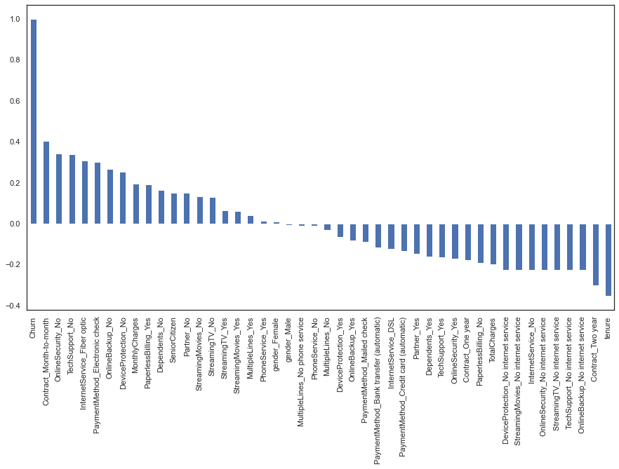
Let us analyze the results of this correlation graph. From right to left, we observe churn attribute, that as expected, has a correlation of 1 with itself. Other attributes that have a high correlation with churn are contracts, online security, and technical support. In another hand, from left to right, two-year contracts and tenure, as the customers are retained, have a negative correlation with churn.
Now, depending on the interest of our study, we can plot various variables in our dataset, using the matplotlib.ticker library. For demonstration purposes, we would like to plot the gender variable in our dataset and see the percentage of men and women customers. This is achieved with the following code:
And outputs the following graph:
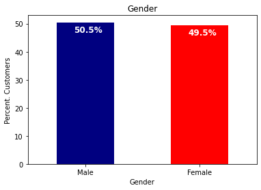
Let us take another example, and plot our customers by senior citizenship, using the a similar code:
To obtain the following pie chart:
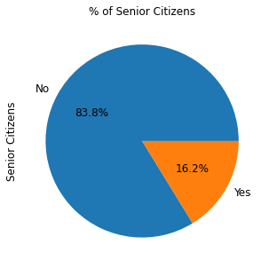
Now we have our data ready, it is time to predict the churn of customers. In the next section, we describe the machine learning model used in this article to predict the churn rate.
Machine Learning Model
Before building the model, we must recall that we have already transformed all categorical variables into dummy attributes. This process will make the implementation of machine learning easier for all the attributes of the dataset, and we will not have to use multiple functions. In fact, we will be using this dummy data frame that we created in earlier sections, and we will also scale the variables to a value between 0 and 1, to be more suitable for the algorithm. These two operations are achieved with the following code:
In order to use the machine learning algorithm, we will have to randomly split the dataset to provide both the training and the testing data. This is achieved with the following lines of code:
For the purpose of this study, we will use a logistic regression model to predict the churn rate. We will begin by fitting the regression model to our training data.
Model Evaluation
At this moment, we are ready to run the model. To do that, we use the predict() function from the LogisticRegression library to make a prediction on the actual testing data. We can observe that the obtained accuracy is 80% of correctly classified instances.
0.8075829383886256
Now, we will see how to interpret the confusion matrix:
We can observe from the results that 1418 and 286 were respectively the true positives and false positives, or the correctly classified instances, in this case, the likelihood of a customer to churn. The sum of these instances is 1704, which represents 80% of the total 2110 instances.
In this article, we have seen predicted churn in the telecommunication industry using machine learning algorithms in Python. As a database to store our data, we used GridDB.
In case you would like to take this article a step further, you can try with other classification algorithms that can be executed in a similar way to the example provided in this article. For more details, visit the open source notebook.
- https://www.heavy.ai/blog/strategies-for-reducing-churn-rate-in-the-telecom-industry
- https://www.kaggle.com/bandiatindra/telecom-churn-prediction/notebook
If you have any questions about the blog, please create a Stack Overflow post here https://stackoverflow.com/questions/ask?tags=griddb . Make sure that you use the “griddb” tag so our engineers can quickly reply to your questions.
Leave a Reply Cancel reply
Your email address will not be published. Required fields are marked *
This site uses Akismet to reduce spam. Learn how your comment data is processed .
IMAGES
VIDEO
COMMENTS
Telecom churn case study where, Based on customer behavior (such as the monthly bill, internet usage, etc.) to predict whether a particular customer will switch to another telecom provider or not (i.e. churn or not). Visualised data and provided some insights on the same. The case study has the following files:
Problem Statement: In the telecom industry, customers are able to choose from multiple service providers and actively switch from one operator to another. In this highly competitive market, the telecommunications industry experiences an average of 15-25% annual churn rate. Given the fact that it costs 5-10 times more to acquire a new customer than to retain an existing one, customer retention ...
Telecom Churn Case Study Problem Statement Business Problem Overview. In the telecom industry, customers are able to choose from multiple service providers and actively switch from one operator to another. In this highly competitive market, the telecommunications industry experiences an average of 15-25% annual churn rate.
Telecom Churn Case Study. # Load the given files. # Collate the 3 files in a single file. # Understand the structure of the collated file. # Make bar charts to find interesting relationships between variables. # Make Box plots for numeric variables to look for outliers. # Impute the missing values, and perform the outlier treatment.
We're told by our colleagues at the hypothetical company that customer churn is at 50% within 3 months. That means that within 3 months of a set of customers that sign up for the paid product, by the end of 3 months half of them will have cancelled. This is an urgent problem we need to help fix with machine learning!
Churn rate for customers with both Phone and Internet service is about 32.9% and Churn rate for customers with either Phone or Internet Service is 26.7%. Customers with internet service and online ...
In this highly competitive market, the telecommunications industry experiences an average of 15-25% annual churn rate. Given the fact that it costs 5-10 times more to acquire a new customer than to retain an existing one, customer retention has now become even more important than customer acquisition. For many incumbent operators, retaining ...
churn currently ranges from 5% to 32% per year[11]. Usually if a customer leaves the company, he or she will not come back within one year. Thus an over 20% of the churn rate would be a heavy loss for the company. However, with telecom companies become more digitized, more insights have been generated.
In this study, a customer churn model is provided for the existing secondary data based case study from Kaggle.com and Github web sites to work on the metrics evaluation. The results show that the use-case model built based on machine learning technique is performing better.
Presentation of final project:Data : https://www.kaggle.com/competitions/telecom-churn-case-study-hackathon-c43/dataGitHub: https://github.com/pmgsalvado/Cou...
Something went wrong and this page crashed! If the issue persists, it's likely a problem on our side. Unexpected token < in JSON at position 4. keyboard_arrow_up. content_copy. SyntaxError: Unexpected token < in JSON at position 4. Refresh. Explore and run machine learning code with Kaggle Notebooks | Using data from telecom_churn.
Customer churn is a major problem and one of the most important concerns for large companies. Due to the direct effect on the revenues of the companies, especially in the telecom field, companies are seeking to develop means to predict potential customer to churn. Therefore, finding factors that increase customer churn is important to take necessary actions to reduce this churn. The main ...
To reduce customer churn, telecom companies need to predict which customers are at high risk of churn. In this project, we analysed customer-level data of a leading telecom firm, build predictive models to identify customers at high risk of churn and identify the main indicators of churn. You can also access the Live web-app here.
The churn rate in the telecom industry is approximately 1.9% every month and can raise to 67% every year. ... Then we introduce the dataset used in this study. We also import the necessary Python libraries to load the dataset. ... or the correctly classified instances, in this case, the likelihood of a customer to churn. The sum of these ...
Case Study: Churn Prediction 4 minute read Business Problem Overview. In the telecom industry, customers are able to choose from multiple service providers and actively switch from one operator to another. In this highly competitive market, the telecommunications industry experiences an average of 15-25% annual churn rate.
Telecom Churn Case Study Business problem overview. In the telecom industry, customers are able to choose from multiple service providers and actively switch from one operator to another. In this highly competitive market, the telecommunications industry experiences an average of 15-25% annual churn rate. Given the fact that it costs 5-10 times ...
GitHub is where people build software. More than 100 million people use GitHub to discover, fork, and contribute to over 420 million projects. ... Telecom-Churn-Case-Study. churn-user-prediction churn-analysis telecom-churn-prediction telecom-churn-analysis Updated Apr 29, 2023;
Explore and run machine learning code with Kaggle Notebooks | Using data from Telecom Churn Case Study Hackathon
Something went wrong and this page crashed! If the issue persists, it's likely a problem on our side. Unexpected token < in JSON at position 4. keyboard_arrow_up. content_copy. SyntaxError: Unexpected token < in JSON at position 4. Refresh. Cleaned Orange Telecom Customer Churn Dataset.
GitHub is where people build software. More than 100 million people use GitHub to discover, fork, and contribute to over 420 million projects. ... Telecom-Churn-Case-Study. churn-user-prediction churn-analysis telecom-churn-prediction telecom-churn-analysis Updated Apr 29, 2023;
In the telecom industry, customers are able to choose from multiple service providers and actively switch from one operator to another. In this highly competitive market, the telecommunications industry experiences an average of 15-25% annual churn rate.
If the issue persists, it's likely a problem on our side. Unexpected token < in JSON at position 4. keyboard_arrow_up. content_copy. SyntaxError: Unexpected token < in JSON at position 4. Refresh. Identify customers at high risk of churn and the main indicators of churn.